
1. Introduction
It can be said that Deep Learning, which is built upon artificial neural networks, has become a core technical foundation of many modern artificial intelligence systems, particularly effective in image recognition and natural language processing tasks. Among these models, the Multi-layer Perceptron (MLP) plays the role of a foundational architecture, serving as the basis for the development of more complex models in the future.
An MLP is constructed from fundamental components such as the Perceptron, weights, bias, activation functions, and is organized in a multi-layer structure. Through the mechanisms of forward propagation and backpropagation, combined with Gradient Descent, the model is able to learn from data and gradually improve the accuracy of its predictions. A clear understanding of each of these components is a necessary condition not only for using the model, but also for explaining, analyzing, and adjusting it to best fit a given problem.
Based on this requirement, the group selected the topic Building an MLP model for handwritten digit prediction, focusing on designing and analyzing a Multi-layer Perceptron model to predict handwritten digits from 0 to 9. This is a classic problem in the field of machine learning, commonly used as an introductory example, as it is simple enough to clearly illustrate the nature of the model while still being realistic enough to reflect the complete process of building a machine learning system.
Objectives of the Project
This report aims to achieve the following main objectives:
- Present the fundamental concepts of the Perceptron and MLP, including weights, bias, activation functions, and layer structure.
- Clarify the operating mechanism of neural networks through forward propagation and backpropagation.
- Apply theoretical knowledge to build an MLP model for the handwritten digit recognition task.
- Describe the model implementation process, from input data and training to result evaluation.
- Develop the ability to connect theory - algorithms - practical implementation using programming tools (PyTorch).
Through this, the report helps readers build a solid foundation in artificial neural networks, thereby creating a basis for approaching more complex Deep Learning models in real-world applications.
2. Perceptron
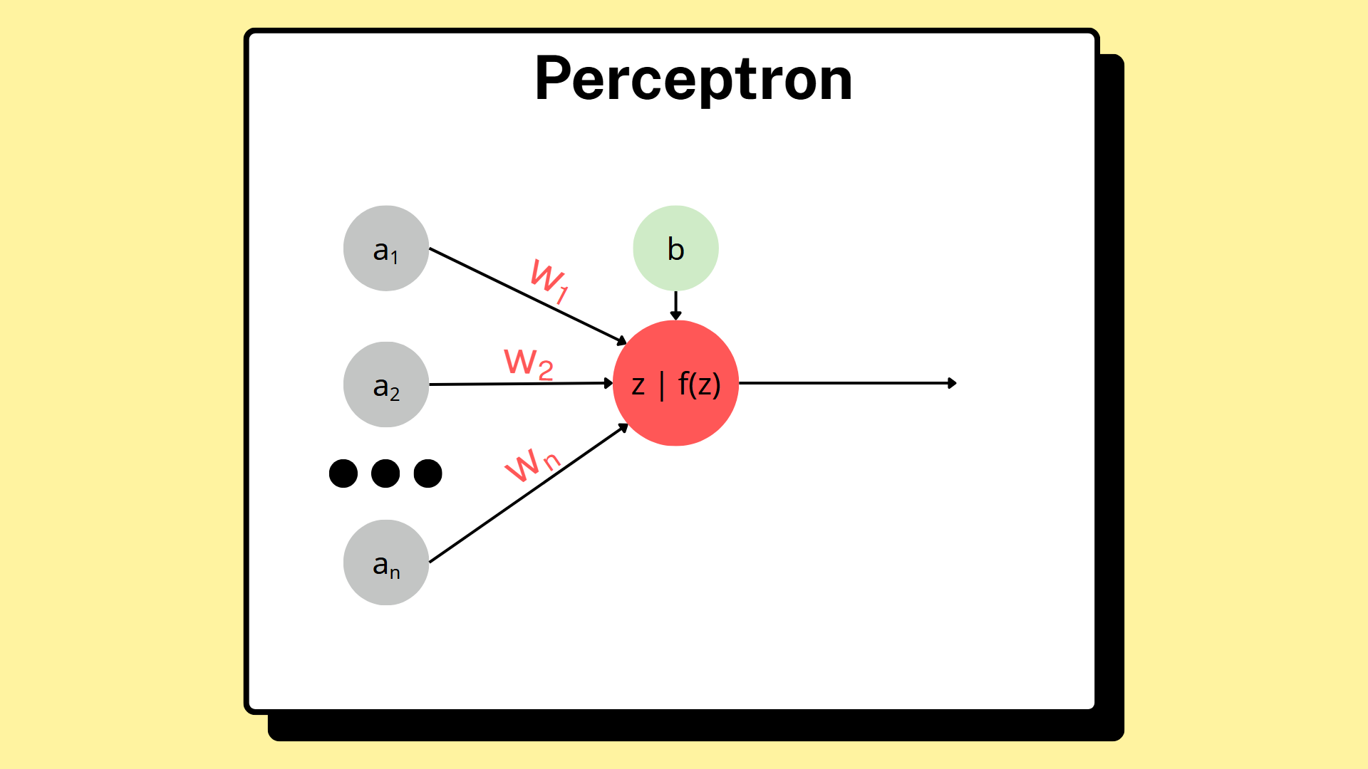
The Perceptron is one of the earliest algorithms designed to solve the binary classification problem. In addition, it serves as the foundation of modern artificial neural networks (ANNs) and is the basic building block for more complex deep learning models. It operates by combining input data (inputs) with corresponding weights, adding a bias, and then producing an output through the use of an activation function.
2.1. Weights and Bias
Weights are parameters that determine the importance of each input feature in making the final prediction. An input associated with a larger weight has a stronger influence on the final output.
The bias is a value added to the weighted sum of the inputs. It is introduced to shift the decision boundary and adjust the prediction in a more flexible manner.
2.2. Activation Function
An activation function is a mathematical function applied to the linear output of a neuron. It is a crucial component of neural networks, as it introduces non-linearity into the model. This non-linearity allows neural networks to learn and represent complex patterns found in real-world data. Without activation functions, regardless of how many layers a neural network has, it would be equivalent to a simple linear regression model. In that case, the model would only be able to learn simple linear relationships between inputs and outputs.
Below is a table introducing several common activation functions:
| Symbol | Full Name | Formula |
|---|---|---|
| Linear | Linear (Identity) Function | $$f(x) = x$$ |
| Step | Binary Step Function | $$f(x)=\begin{cases}1 & x \ge 0 \\ 0 & x < 0\end{cases}$$ |
| $\sigma(x)$ | Sigmoid Function | $$f(x)=\frac{1}{1+e^{-x}}$$ |
| $\tanh(x)$ | Hyperbolic Tangent Function | $$f(x)=\frac{e^x-e^{-x}}{e^x+e^{-x}}$$ |
| ReLU | Rectified Linear Unit Function | $$f(x)=\begin{cases}x & x>0 \\ 0 & x\le 0\end{cases}$$ |
| LReLU | Leaky Rectified Linear Unit Function | $$f(x)=\begin{cases}x & x>0 \\ \alpha x & x\le 0\end{cases}$$ |
| Softplus | Softplus Function | $$f(x)=\ln(1+e^x)$$ |
| Softmax | Softmax Function | $$f(x_i)=\frac{e^{x_i}}{\sum_{j=1}^{K} e^{x_j}}$$ |
Choosing an appropriate activation function is a critical step in neural network design. It not only affects the model's ability to learn meaningful features from the training data, but also influences the learning speed and the model's ability to generalize when deployed in real-world applications.
3. Layer
In a Multi-Layer Perceptron (MLP), a layer is the functional unit of the project that performs step-by-step data transformations during the learning process. Dividing the network into multiple layers is not simply a chosen technique but stems from the need to extend the model's representational capabilities for linear feature delivery systems.
Neurons within the same layer share the same maximum path length from the input layer.
4. Single-layer Perceptron
4.1. Structure of the Single-layer Perceptron
A Single-layer Perceptron is the simplest form of a neural network. It consists only of an input layer and a single perceptron layer directly connected to the output, with no hidden layers in between. Structurally, it includes four main components that operate sequentially.
The first component is the input vector, also known as the feature vector. It is represented as $\mathbf{x} = [x_1, x_2, ..., x_m]^T$. For example, when deciding whether to go to the movies, you might consider the weather $x_1$, your mood $x_2$, the amount of money you have $x_3$, and the quality of the movie $x_4$. Each feature represents one dimension of information that the model uses to make a prediction.
The second component is the set of weights, which measure the importance of each feature and are represented as $\mathbf{w} = [w_1, w_2, ..., w_m]^T$. For instance, if movie quality is the most important factor for you, it may have a higher weight $x_4 = 0.5$, while weather might be less important and thus have a lower weight $x_1 = 0.1$. These weights are what the model learns from data: they are initially randomized and then gradually adjusted during training to reflect the true importance of each feature.
Next is the bias $b$ - which acts as a decision threshold. Conceptually, a large positive bias corresponds to being more easily agreeable, while a negative bias reflects a stricter decision tendency. Mathematically, the bias shifts the decision boundary independently of the input values.
Finally, there is the activation function, which produces the final decision. In the classical perceptron, the activation function is usually the step function. This simple function outputs 1 if $z$ is greater than or equal to $0$, and $0$ (or $-1$) if $z$ less than $0$.
$$ f(z) = \begin{cases} 1 & , z \ge 0\\ 0 & , z \lt 0 \end{cases} $$
4.2. Computation Process
The computation process consists of three steps:
-
Step 1: Receive the input vector $\mathbf{x}$.
-
Step 2: Compute the weighted sum $z = w_1x_1 + w_2x_2 + ... + w_2x_2 + b$. Or in vector form: $z = \mathbf{w}^T \mathbf{x} + b$.
-
Step 3: Apply the activation function to obtain the output $y = f(z)$.
The entire process involves only simple multiplication and addition, making it extremely fast, yet capable of performing the most basic form of classification in machine learning.
Practical Application
For example, suppose we want to model the rule that we are allowed to go out if and only if we have finished our homework and received permission from our parents. This rule is essentially an AND function. The AND function output $y=1$ only when both $x_1$ and are equal to 1. The truth table is as follows:
| $x_1$ (homework done) | $x_2$ (permission granted) | $y$ |
|---|---|---|
| 0 | 0 | 0 |
| 0 | 1 | 0 |
| 1 | 0 | 0 |
| 1 | 1 | 1 |
To represent the AND function using a Single-layer Perceptron, we set the weights and bias as follows: $w_1 = 1$, $w_2 = 1$, $b = -1.5$.
When $x_1 = 0$ and $x_2 = 0$, this corresponds to the case where the homework has not been completed and permission has not been granted. We have $z = 1 \times 0 + 1 \times 0 - 1.5 = -1.5$. Since $z \lt 0$, $y = f(z) = 0$. Therefore, we are not allowed to go out.
When $x_1 = 0$ and $x_2 = 1$, this corresponds to the case where the homework has not been completed but permission has been granted. We have $z = 1 \times 0 + 1 \times 1 - 1.5 = -0.5$. Since $z \lt 0$, $y = f(z) = 0$. Therefore, we are not allowed to go out.
When $x_1 = 1$ and $x_2 = o$, this corresponds to the case where the homework has been completed but permission has not been granted. We have $z = 1 \times 1 + 1 \times 0 - 1.5 = -0.5$. Since $z \lt 0$, $y = f(z) = 0$. Therefore, we are not allowed to go out.
In the final case, when $x_1 = 1$ and $x_2 = o$, this corresponds to the case where the homework has been completed and permission has been granted. We have $z = 1 \times 1 + 1 \times 1 - 1.5 = 0.5$. Since $z \gt 0$, $y = f(z) = 1$.Therefore, we are allowed to go out.
4.3. Limitations of the Single-layer Perceptron
A Single-layer Perceptron can only classify linearly separable data - meaning that a straight line (or hyperplane) can be drawn to separate the two classes.
A classic failure occurs when attempting to represent the XOR function using a Single-layer Perceptron. The XOR function outputs $y = 1$ if and only if $x_1$ and $x_2$ are different. The truth table of the XOR function is shown below:
| $x_1$ | $x_2$ | $y$ |
|---|---|---|
| 0 | 0 | 0 |
| 0 | 1 | 1 |
| 1 | 0 | 1 |
| 1 | 1 | 0 |
When these four points are plotted on a plane, the two points with $y = 1$ are $(0,1)$ and $(1,0)$ lie at opposite corners, while the two points with $y = 1$ are $(0,0)$ and $(1,1)$ occupy the other opposite corners. They form an interleaving “X” pattern, for which no straight line can separate the two classes. Any straight line will inevitably intersect both classes.
Historical impact: In 1969, Minsky and Papert proved that a single-layer perceptron cannot learn the XOR function. This result led to the first “AI winter,” during which funding dried up, researchers left the field, and AI research stagnated for nearly two decades.
5. Multi-Layer Perceptron (MLP)
5.1. Architecture of the MLP
As discussed in the previous section, a single-layer perceptron is inherently limited to learning linear decision boundaries. While such models are simple and interpretable, they are fundamentally incapable of representing complex non-linear relationships that commonly arise in real-world data.
The Multi-Layer Perceptron (MLP) addresses this limitation not by changing the basic computational unit, but by organizing perceptrons into a structured hierarchy of layers. This architectural extension enables the model to represent increasingly complex functions through the composition of simpler transformations. Before examining how information flows through the network or how the model is trained, it is essential to first understand this architectural structure.
5.1.1. High-Level View of MLP Architecture
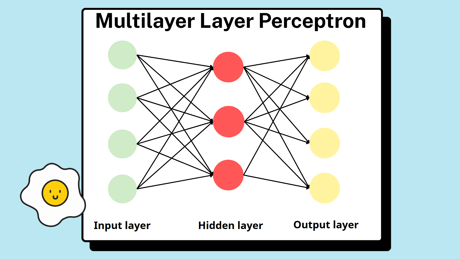
From an architectural standpoint, an MLP is a feedforward neural network composed of multiple layers of neurons arranged sequentially. It consists of three fundamental components:
- Input layer
- One or more hidden layers
- Output layer
Neurons in one layer are typically fully connected to neurons in the subsequent layer, forming a directed acyclic structure. Information moves strictly in one direction—from the input layer toward the output layer—following the connections defined by the architecture.
The defining feature of the MLP is the presence of hidden layers, which allow the network to transform raw inputs into progressively richer internal representations. This layered organization is what distinguishes MLPs from single-layer models and enables their expressive power.
5.1.2. Core Architectural Components
Input Layer
The input layer serves as the interface between raw data and the neural network. Its role is to receive the input features and pass them directly to the first hidden layer.
Importantly, the input layer does not perform any learning or transformation. Its dimensionality is determined entirely by the chosen representation of the input data.
Hidden Layers
Hidden layers constitute the representational core of the MLP. Each hidden layer contains a set of neurons that apply learned transformations to the outputs of the preceding layer.
By stacking multiple hidden layers, the MLP forms a hierarchy of representations. Earlier layers tend to capture simpler patterns, while deeper layers combine these patterns into more abstract features. The number of hidden layers and the number of neurons within each layer are architectural design choices that directly influence the model’s capacity to represent complex functions.
Output Layer
The output layer produces the final output of the network. Its structure depends on the type of task being addressed, such as regression or classification.
From an architectural perspective, the output layer completes the transformation pipeline by mapping the final hidden representation to the model’s output space.
5.1.3. Neuron-Level Computation (Architectural Perspective)
At the architectural level, each neuron in a hidden or output layer is defined by two conceptual elements:
- A linear transformation of its inputs, parameterized by a weight matrix $W^{(l)}$ and a bias vector $b^{(l)}$
- A non-linear activation function, producing an activation vector $a^{(l)}$
This relationship can be expressed symbolically as:
$$ a^{(l)} = f\left( W^{(l)T} a^{(l-1)} + b^{(l)} \right) $$
At this stage, it is sufficient to recognize that this repeated structural composition-rather than the computational process itself-is what gives the MLP its capacity to represent complex, non-linear relationships.
With the MLP architecture defined and the input dimensionality fixed by the chosen data representation, the next step is to examine how information flows through this structure via forward propagation.
5.2. Forward Propagation
The most common algorithms for optimizing MLP models are still Gradient Descent and its variations (Adam, Momentum, RMSProp, etc.). Their common feature is that they all require calculating the predicted output vector $\mathbf{\hat{y}}$ corresponding to the feature vector $\mathbf{x}$.
This step is performed by calculating the activations at each layer, sequentially from front to back. Therefore, it is called forward propagation.
Specifically, let $\mathbf{a^{(0)} = \mathbf{x}}$ be the input. For each level $l = 1, 2, 3, ..., L$ we have:
$$\mathbf{z}^{(l)} = \mathbf{W}^{(l)T} \mathbf{a}^{(l-1)} + \mathbf{b}^{(l)},$$
$$\mathbf{a}^{(l)} = f_l(\mathbf{z}^{(l)}).$$
At the output level:
$$\mathbf{\hat{y}} = \mathbf{a}^{(L)}.$$
In there:
- $\mathbf{x} \in \mathbb{R}^{d^{0}}$ is the feature vector.
- $\mathbf{a}^{(0)} = \mathbf{x}$ is the activation vector at the input layer.
- $L$ is the total number of layers in the model.
- $l \in \{1,2,...,L\}$ is the index of the layers in the model.
- $d^{(l)}$ is the total number of neurons at level $l$.
- $\mathbf{W}^{(l)} \in \mathbb{R}^{d^{(l-1)}} \times \mathbb{R}^{d^{(l)}}$ is the weight matrix at level $l$.
- $\mathbf{W}^{(l)T} \in \mathbb{R}^{d^{(l)}} \times \mathbb{R}^{d^{(l-1)}}$ is the transpose matrix of $\mathbf{W}^{(l)}$.
- $\mathbf{b}^{(l)} \in \mathbb{R}^{d^{(l)}}$ is the deviation vector at level $l$.
- $\mathbf{z}^{(l)} \in \mathbb{R}^{d^{(l)}}$ is the pre-activation vector at level $l$.
- $f_l(\cdot) \in \mathbb{R}^{d^{(l)}} \mapsto \mathbb{R}^{d^{(l)}}$ is the activation function at layer $l$.
- $\mathbf{a}^{(l)} \in \mathbb{R}^{d^{(l)}}$ is the activation vector at level $l$.
- $\mathbf{\hat{y}} = \mathbf{a}^{(L)}$ is the output value of the model.
When we train a model with $N$ samples at the same time, we only need to arrange the feature vectors $x_n$ horizontally to form the matrix $X \in \mathbb{R}^{d^{(0)} \times N}$. Similarly, the matrix $Y \in \mathbb{R}^{d^{(L)} \times N}$ consists of $N$ result vectors $y_n$ arranged side by side.
Each vector $x_n$ in $X$, through forward propagation, creates activation vectors $a_n$ equivalent to the columns of $A^{(l)} \in \mathbb{R}^{d^{(l)} \times N}$. We get:
$$ \mathbf{A^{(0)} = \mathbf{X}}, $$
$$\mathbf{Z}^{(l)} = \mathbf{W}^{(l)T} \mathbf{A}^{(l-1)} + \mathbf{b}^{(l)},$$
$$\mathbf{A}^{(l)} = f_l(\mathbf{Z}^{(l)}),$$
$$\mathbf{\hat{Y}} = \mathbf{A}^{(L)}.$$
5.3. Backpropagation
After finding $\mathbf{\hat{y}}$, the next step in gradient-based optimization algorithms (Gradient Descent, Adam,...) is to find the derivative of the loss function with respect to the weights and biases.
A common method for calculating gradients is the backpropagation algorithm. The main idea of this method is to initially calculate the gradient at the last layer, then use the chain rule to find the gradient at the immediately preceding layer. The algorithm repeats this step, successively calculating all the derivatives at each layer in order from last to first (from the output layer to the input layer).
Let's assume that $J(\theta, \mathbf{X}, \mathbf{Y})$ is the loss function, where $\theta$ is the set of all weight matrices and bias vectors of each layer, $\theta \in \{\mathbf{W}^{(1)}, \mathbf{b}^{(1)}, \mathbf{W}^{(1)}, \mathbf{b}^{(1)}, ..., \mathbf{W}^{(L)}, \mathbf{b}^{(L)}\}$. $\mathbf{X}, \mathbf{Y}$ are the sets of training pairs $\mathbf{x}, \mathbf{y}$. To calculate the derivative of $J$ with respect to $\mathbf{W}$ and $\mathbf{b}$, we need to calculate it for $l=1,2,...,L$ in turn:
$$ \frac{\partial J}{\partial \mathbf{W}^{(l)}}, \; \frac{\partial J}{\partial \mathbf{b}^{(l)}}. $$
5.3.1. Representing the derivative in terms of each component
This is how to represent the component-wise derivative of $\mathbf{W}^{(l)}, \mathbf{b}^{(l)}$.
Specifically, at the output layer we have the following derivatives:
$$ \frac{\partial J}{\partial w_{ij}^{(L)}} = \frac{\partial J}{\partial z_{j}^{(L)}} \frac{\partial z_{j}^{(L)}}{\partial w_{ij}^{(L)}} = e_{j}^{(L)} a_{i}^{(L-1)}, $$
$$ \frac{\partial J}{\partial b_{j}^{(L)}} = \frac{\partial J}{\partial z_{j}^{(L)}} \frac{\partial z_{j}^{(L)}}{\partial b_{j}^{(L)}} = e_{j}^{(L)}. $$
In this case, $e_{j}^{(L)} = \frac{\partial J}{\partial z_{j}^{(L)}}$ is an easily calculable quantity, and $\frac{\partial z_{j}^{(L)}}{\partial w_{ij}^{(L)}} = a_{i}^{(L-1)}$ and $\frac{\partial z_{j}^{(L)}}{\partial b_{j}^{(L)}} = 1$ because $z_{j}^{(L)} = \mathbf{w}_{j}^{(L)T} \mathbf{a}^{(L)} + b_{j}^{(L)}$.
For hidden layers, the derivative is calculated as:
$$ \begin{aligned} \frac{\partial J}{\partial w_{ij}^{(l)}} &= \frac{\partial J}{\partial z_{j}^{(l)}} \frac{\partial z_{j}^{(l)}}{\partial w_{ij}^{(l)}} \\ &= e_{j}^{(l)} a_{i}^{(l-1)}, \end{aligned} $$
with:
$$ \begin{aligned} e_{j}^{(l)} &= \frac{\partial J}{\partial z_{j}^{(l)}} = \frac{\partial J}{\partial a_{j}^{(l)}} \frac{\partial a_{j}^{(l)}}{\partial z_{j}^{(l)}} \\ &= \left( \sum_{k=1}^{d^{(l+1)}} \frac{\partial J}{\partial z_{k}^{(l+1)}} \frac{\partial z_{k}^{(l+1)}}{\partial a_{j}^{(l)}} \right) f_{l}^{\prime}(z_{j}^{(L)}) \\ &= \left( \sum_{k=1}^{d^{(l+1)}} e_{k}^{(l+1)} w_{jk}^{(l+1)} \right) f_{l}^{\prime}(z_{j}^{(L)}) \\ &= \left( \mathbf{w}_{j:}^{(l+1)} \mathbf{e}^{(l+1)} \right) f_{l}^{\prime}(z_{j}^{(L)}), \end{aligned} $$
where $\mathbf{e}^{(l+1)} = [e_{1}^{(l+1)}, e_{2}^{(l+1)}, ..., e_{d^{(l+1)}}^{(l+1)}]^T \in \mathbb{R}^{d^{(l+1)} \times 1}$ and $\mathbf{w}_{j:}^{(l+1)}$ is the j-th column of the matrix $\mathbf{W}^{(l+1)}$.
Similarly, we have:
$$ \frac{\partial J}{\partial b_{j}^{(l)}} = \frac{\partial J}{\partial z_{j}^{(l)}} \frac{\partial z_{j}^{(l)}}{\partial b_{j}^{(l)}} = e_{j}^{(l)}. $$
5.3.2. Representing Derivatives as Vectors
To speed up the algorithm's computation, we need to convert the derivative expressions into vector or matrix form. For Stochastic Gradient Descent, we will represent them as vectors.
At the output stage, we need to calculate:
$$ \mathbf{e}^{(L)} = \frac{\partial J}{\partial \mathbf{z}^{(L)}}, $$
$$ \frac{\partial J}{\partial \mathbf{W}^{(L)}} = \mathbf{a}^{(L-1)} \mathbf{e}^{(L)T}, $$
$$ \frac{\partial J}{\partial \mathbf{b}^{(L)}} = \mathbf{e}^{(L)}. $$
For the hidden layers, we have:
$$ \mathbf{e}^{(l)} = \left( \mathbf{W}^{(l+1)} \mathbf{e}^{(l+1)} \right) \odot f_l^\prime(z^{(l)}), $$
$$ \frac{\partial J}{\partial \mathbf{W}^{(l)}} = \mathbf{a}^{(l-1)} \mathbf{e}^{(l)T}, $$
$$ \frac{\partial J}{\partial \mathbf{b}^{(l)}} = \mathbf{e}^{(l)}. $$
In this case, $\odot$ is the element-wise/Hadamard product operation.
5.3.3. Representing Derivatives as Matrices
If we are using Batch or Mini-batch Gradient Descent, we need to represent them as matrices.
Let's assume that for each training period we use $N$ samples. Then the matrix $X \in \mathbb{R}^{d^{(0)} \times N}$ will have the form $N$ feature vectors $x_n$ arranged consecutively in rows. Similarly, the matrix $Y \in \mathbb{R}^{d^{(L)} \times N}$ consists of $N$ result vectors $y_n$ arranged next to each other.
Each vector in $X$ will have its activation vectors calculated, with errors equivalent to the columns of $A^{(l)} \in \mathbb{R}^{d^{(l)} \times N}$ and $E^{(l)} \in \mathbb{R}^{d^{(l)} \times N}$.
At the output stage, we need to calculate:
$$ \mathbf{E}^{(L)} = \frac{\partial J}{\partial \mathbf{Z}^{(L)}}, $$
$$ \frac{\partial J}{\partial \mathbf{W}^{(L)}} = \mathbf{A}^{(L-1)} \mathbf{E}^{(L)T}, $$
$$ \frac{\partial J}{\partial \mathbf{b}^{(L)}} = \sum_{n=1}^{N} \mathbf{e}_n^{(L)}. $$
For the hidden layers, we have:
$$ \mathbf{E}^{(l)} = \left( \mathbf{W}^{(l+1)} \mathbf{E}^{(l+1)} \right) \odot f_l^\prime(z^{(l)}), $$
$$ \frac{\partial J}{\partial \mathbf{W}^{(l)}} = \mathbf{A}^{(l-1)} \mathbf{E}^{(l)T}, $$
$$ \frac{\partial J}{\partial \mathbf{b}^{(l)}} = \sum_{n=1}^{N} \mathbf{e}_n^{(l)}. $$
5.4. Updating Parameters
After calculating the derivative, gradient-based optimization algorithms adjust the parameters in the opposite direction to the gradient. Assuming the chosen optimization algorithm is Gradient Descent, the model parameters at iteration $t$ are:
$$ \theta^{(t)} = \theta^{(t-1)} - \eta \frac{\partial J}{\partial \theta^{(t-1)}}, \;\;\; \theta \in \{\mathbf{W}^{(1)}, \mathbf{b}^{(1)}, \mathbf{W}^{(1)}, \mathbf{b}^{(1)}, ..., \mathbf{W}^{(L)}, \mathbf{b}^{(L)}\}, $$
where $\eta$ is the learning rate.
6. Project Description
6.1. Objective
The team's goal was to create a simple website that takes an RGB image as input with two primary colors, one for the background and the other for a number from 0 to 9. The system would then return the expected result for that number.
6.2. Implementation
6.2.1. Process Dataset
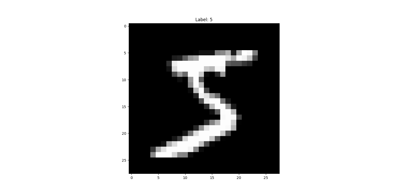
To train a handwritten digit classification model, the most popular dataset currently used is the MNIST dataset – a collection of 70,000 grayscale images of black and white handwritten digits. Each image has 28 pixels in both length and width, totaling $28 \times 28 = 784$ pixels. Each pixel has a value from 0 to 255, with 0 representing black – the background of the image; and 255 representing white – the dominant color of the handwritten digits.
Each image is paired with a label that accurately represents the numerical value shown in that image, together creating a sample – used for training or evaluating the model.
To improve the model's efficiency, the input data was scaled from 0 to 255 to 0 to 1. Fortunately, PyTorch provides specialized functions for this purpose.
import os
import torch
import torch.nn as nn
import torch.nn.functional as F
from torch.utils.data import DataLoader
from torchvision import datasets, transforms
from tqdm.auto import tqdm

transform = transforms.Compose([
    transforms.ToTensor()
])

root = os.path.join(os.getcwd(), "data")
train_ds = datasets.MNIST(root=root, train=True, download=True, transform=transform)
val_ds   = datasets.MNIST(root=root, train=False, download=True, transform=transform)
Specifically, the .ToTensor method converts image data to tensors and changes the pixel values from 0-255 to 0-1. The variables train_ds and val_ds represent the training and testing sets, respectively.
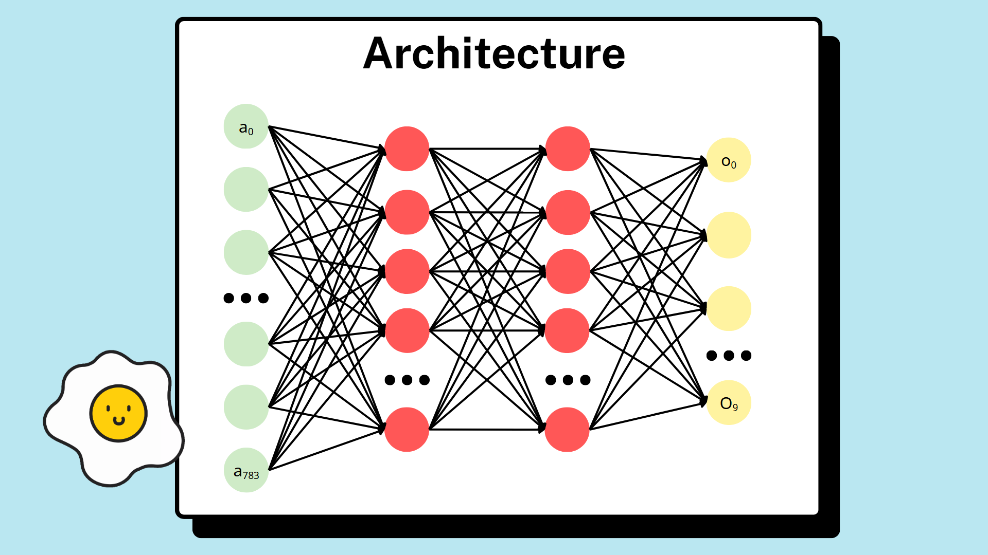
6.2.2. MLP Model Architecture
The simplified MLP model that our team chose to solve the problem has a structure consisting of 1 input layer, 2 hidden layers, and 1 output layer.
The input layer's task is to flatten a 2D image into a one-dimensional array, conforming to the MLP model architecture. This means there are 784 neurons in this layer (each neuron for one pixel). The two subsequent hidden layers both use ReLU as the activation function, unlike the output layer which uses the Softmax function. The output layer has 10 neurons, each with a value corresponding to the probability of a digit (0-9) appearing in the image. In other words, the value of the first neuron represents the probability that the digit in the image is 0; the value of the second neuron represents the probability that the digit in the image is 1; and so on. The model will return the result based on the highest probability.
DEVICE = torch.device("cuda" if torch.cuda.is_available() else "cpu")

INPUT_SIZE = 28 * 28
HIDDEN_SIZE_1 = 512
HIDDEN_SIZE_2 = 256
OUTPUT_SIZE = 10

model = nn.Sequential(
    nn.Flatten(),
    nn.Linear(INPUT_SIZE, HIDDEN_SIZE_1),
    nn.ReLU(),
    nn.Linear(HIDDEN_SIZE_1, HIDDEN_SIZE_2),
    nn.ReLU(),
    nn.Linear(HIDDEN_SIZE_2, OUTPUT_SIZE)
).to(DEVICE)
The code above defines the model correctly according to the description above. The only difference is that we have not defined the Softmax activation function for the output layer. This difference exists because the Cross-Entropy loss function, which will be defined in the training section, already has the Softmax activation function built in front of it; therefore, we don't need to define it here.
6.2.3. Training and Testing
To speed up the training and testing process, we did not feed all 60,000 samples directly into the model at once, but instead divided them into batches, each batch size being 64 samples.
BATCH_SIZE = 64

train_loader = DataLoader(train_ds, batch_size=BATCH_SIZE, shuffle=True)
val_loader   = DataLoader(val_ds, batch_size=BATCH_SIZE, shuffle=False)
One of the most popular optimization algorithms for training models is Adam, an improvement on Gradient Descent. It is implemented as follows, where lr is the learning rate.
lr = 1e-3

optimizer = torch.optim.Adam(model.parameters(), lr=lr)
The training and testing functions are defined as follows, respectively:
def train_one_epoch(model, loader, optimizer):
    model.train()
    total, correct, total_loss = 0, 0, 0.0
    for x, y in tqdm(loader, leave=False):
        x, y = x.to(DEVICE), y.to(DEVICE)
        logits = model(x)
        loss = F.cross_entropy(logits, y)
        optimizer.zero_grad()
        loss.backward()
        optimizer.step()
        total_loss += loss.item() * x.size(0)
        preds = logits.argmax(dim=1)
        correct += (preds == y).sum().item()
        total += x.size(0)
    return total_loss / total, correct / total

def evaluate(model, loader):
    model.eval()
    total, correct, total_loss = 0, 0, 0.0
    with torch.no_grad():
        for x, y in loader:
            x, y = x.to(DEVICE), y.to(DEVICE)
            logits = model(x)
            loss = F.cross_entropy(logits, y)
            total_loss += loss.item() * x.size(0)
            preds = logits.argmax(dim=1)
            correct += (preds == y).sum().item()
            total += x.size(0)
    return total_loss / total, correct / total
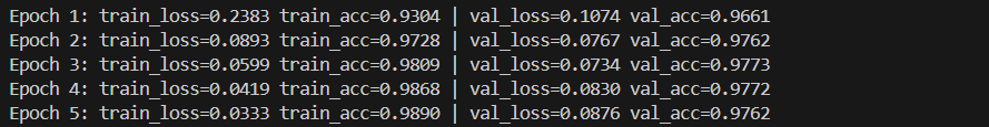
We then train and test the model:
epochs = 5

for ep in range(1, epochs+1):
    t_loss, t_acc = train_one_epoch(model, train_loader, optimizer)
    v_loss, v_acc = evaluate(model, val_loader)
    print(f"Epoch {ep}: train_loss={t_loss:.4f} train_acc={t_acc:.4f} | val_loss={v_loss:.4f} val_acc={v_acc:.4f}")
After the training was complete, we saved the model parameters for use in the system.
PATH = "model.pt"
torch.save(model.state_dict(), PATH)
6.2.4. Process User-Provided Images
Currently, the model has only learned black and white images from the MNIST dataset, while the project's objective is to use RGB images with two primary colors. Therefore, we need to process the images uploaded by the user. The following are the image processing steps:
- Step 1: Convert the image from RGB to black and white.
- Step 2: Resize the image to $28 \times 28$ to fit the model's input.
- Step 3: Invert the colors if the numbers are black on a white background (MNIST images have a black background and white numbers, contrary to the project's requirement).
- Step 4: Clean the image using thresholding, leaving only two values: 0 for black and 255 for white.
- Step 5: Center the digits (in MNIST images, all numbers are centered).
- Step 6: Scale the pixel values from 0 to 255 to 0 to 1, matching the MNIST pixel values used for training the model.
- Step 7: Reshape the image to fit the model's input.
- Step 8: Convert the image to tensor form.
import cv2

def preprocess_for_mnist_pytorch(image):
    # 1. Convert from RGB (Gradio) to Grayscale
    gray = cv2.cvtColor(image, cv2.COLOR_RGB2GRAY)

    # 2. Resize image to 28x28
    resized = cv2.resize(gray, (28, 28), interpolation=cv2.INTER_AREA)

    # 3. Invert color if it's black text on a white background
    corners = [resized[0,0], resized[0,-1], resized[-1,0], resized[-1,-1]]
    if np.mean(corners) > 127:
        resized = cv2.bitwise_not(resized)

    # 4. Otsu Thresholding to clean the image (0 or 255)
    _, clean = cv2.threshold(resized, 127, 255, cv2.THRESH_BINARY + cv2.THRESH_OTSU)

    # 5. Centering
    centered = center_digit(clean)

    # 6. Scale to [0,1]
    scaled = centered.astype('float32') / 255.0

    # 7. Reshape to fit model input
    reshaped = scaled.reshape(1, 1, 28, 28)

    # 8. Convert image to pytorch tensor
    final = torch.from_numpy(reshaped).float()

    return final
With the center_digit function is defined using the below code:
def center_digit(img):
    # img is a 28x28 binary image (white text on a black background)

    # Formula M_{ij} = \sum x^i * y^j * pixel value (brightness)
    # Example m00 = \sum x^0 * y^0 * pixel value = total brightness of the image
    # Similarly m10 = \sum x * pixel value = weighted average brightness according to x
    # Similarly m01 = \sum y * pixel value = weighted average brightness according to y
    M = cv2.moments(img)

    if M['m00'] != 0:
        cx = int(M['m10'] / M['m00']) # x-coordinate of the center (x - horizontal)
        cy = int(M['m01'] / M['m00']) # y-coordinate of the center (y - vertical)

        # Calculate the deviation from the geometric center (14, 14)
        shift_x = 14 - cx
        shift_y = 14 - cy

        # Shift Matrix
        M_shift = np.float32([[1, 0, shift_x], [0, 1, shift_y]])

        # Multiply the pixel coordinates of the image by the shift matrix.
        # If the value is outside the 28*28 range, discard it; cells without information default to 0.
        centered_img = cv2.warpAffine(img, M_shift, (28, 28))

        return centered_img
    return img
6.2.5. Creating an Application
Regarding the predictive model, our team will create a model with the same architecture as the trained model. Then, we will load the parameters from the trained model into this newly created model.
import torch
import torch.nn as nn

INPUT_SIZE = 28 * 28
HIDDEN_SIZE_1 = 512
HIDDEN_SIZE_2 = 256
OUTPUT_SIZE = 10

model = nn.Sequential(
    nn.Flatten(),
    nn.Linear(INPUT_SIZE, HIDDEN_SIZE_1),
    nn.ReLU(),
    nn.Linear(HIDDEN_SIZE_1, HIDDEN_SIZE_2),
    nn.ReLU(),
    nn.Linear(HIDDEN_SIZE_2, OUTPUT_SIZE)
)

# Load parameters from the trained model.
PATH = 'model.pt'
state_dict = torch.load(PATH)

# Load parameters into the new model
model.load_state_dict(state_dict)

# Switch the model to inference mode
model.eval()
For the user interface, the team used the Gradio library. With just a few simple lines of code, they created an interface that looks decent.
import gradio as gr

def predict_number(image):
    if image is None:
        return "You haven't uploaded any images"

    input = preprocess_for_mnist_pytorch(image)
    logit = model(input)
    prediction = logit.argmax(dim=1)
    return f"This is the number: {prediction.item()}"

demo = gr.Interface(
    fn=predict_number,
    inputs=gr.Image(label="Upload your digit image"),
    outputs=gr.Textbox(label="Result"),
    api_name="Predict handwritten digits",
    title="Predict the handwritten digits from 0-9",
    description="Project by team CONQ027, AIO Conquer 2026 program"
)

demo.launch()
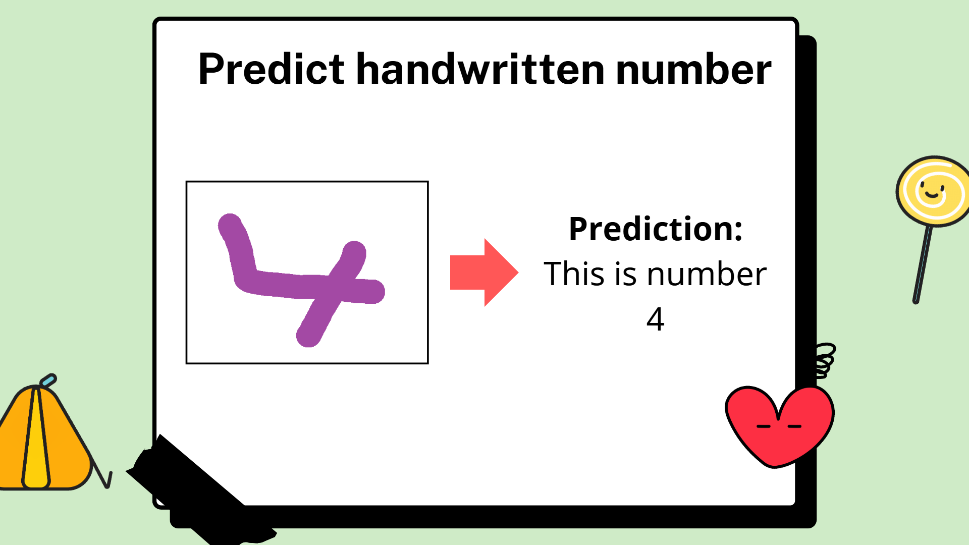
Below is the application interface. On the left, there is a window for users to upload images. After the user uploads the image and clicks "submit", the window on the right will display a prediction of the digits in the image.

7. Conclusion
Although the Multi-Layer Perceptron model is old, simple, and less efficient than later models, the knowledge surrounding it forms the foundation of Deep Learning. The project successfully completed the theoretical research, construction, and experimental testing of a Multi-Layer Perceptron (MLP) model for handwritten digit recognition, thereby helping our team consolidate and better understand the knowledge we had learned.
8. References
Vu, H. T. (2017). Multi-layer Perceptron and Backpropagation. Machine Learning cơ bản. https://machinelearningcoban.com/2017/02/24/mlp
Tran, H. D., Duong, D. T., Dinh, Q. V. (2025). Step-by-Step: Multi-layer Perceptron
Regression. AI VIET NAM. https://lms.aivietnam.edu.vn/api/files/6919b01eeb7f1890ba6b65ce/Documents%2F2025-10%2FM06W03-StudyGuide%26Reading%2FM06W03_Reading_MLP.pdf
Chưa có bình luận nào. Hãy là người đầu tiên!