I. INTRODUCTION
In the world of Data, SQL (Structured Query Language) and Pandas are two "go-to" tools that operate on fundamentally different paradigms.
This article focuses on hands-on coding, helping you directly map familiar SQL clauses to their Pandas equivalents using the Superstore dataset.

Figure 1. Query with SQL and Pandas. (source: gemini)
II. DATA STRUCTURE
2.1. Getting Familiar with Basic SQL Syntax
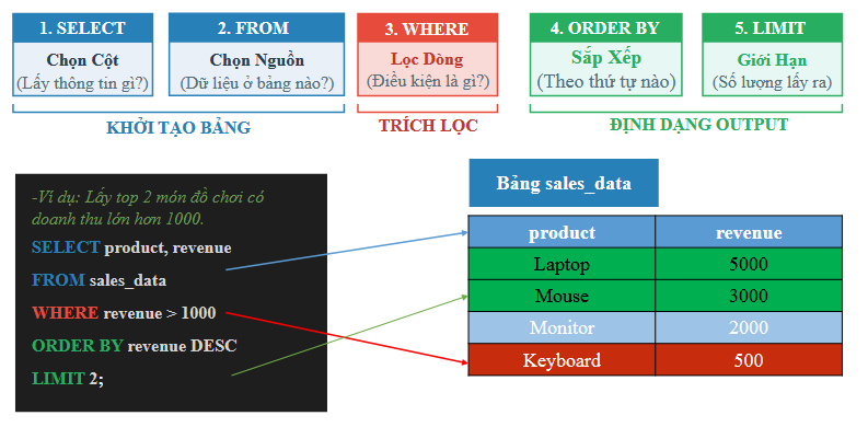
Figure 2. Basic SQL syntax. (source: AIO2026-Pandas&SQL Data Retrieval-Slide 14)
The basic syntax of the SELECT statement, where [...] denotes optional clauses that the user may or may not specify:
SELECT select_list
[ FROM table_source ]
[ WHERE search_condition ]
[ GROUP BY group_by_expression ]
[ HAVING search_condition ]
[ ORDER BY order_expression [ ASC | DESC ] ]
-
SELECT: Lists the data fields (columns) or aggregate functions on those fields to be returned by the query. Note that these fields must exist in the tables specified in theFROMclause. -
FROM: Lists the data tables and/or combines them withJOINoperations for the tables being queried. -
WHERE: Defines the data filtering condition. -
GROUP BY: Groups the data fields to be processed. -
HAVING: Defines the filtering condition applied after grouping and performing group-level calculations, if any. -
ORDER BY: Specifies which data fields to sort by, and whether in ascending (ASC) or descending (DESC) order.
Other important notes:
-
In SQL, the basic processing order of a query statement from left to right is as follows:
FROM,WHERE,GROUP BY,HAVING,SELECT,ORDER BY. -
Operators and functions may vary across different Relational Database Management Systems (RDBMS). For example, the
||operator is used for string concatenation in Oracle, whereas+is used in MS SQL Server. -
Use the special wildcard character
*in theSELECTclause to retrieve all data fields. -
Use
IS NULLorIS NOT NULLto compare against null (empty/unknown) values. -
Use the
LIKEoperator to match string values against a search pattern. -
The
ASclause can be used to rename a displayed field in theSELECTclause or to assign a shorter alias to a table in theFROMclause. -
Use
DISTINCTto eliminate duplicate values. -
Use
LIMITto restrict the number of rows returned.
2.2. Getting Familiar with Basic Pandas Syntax
How Pandas implements the corresponding SQL clauses:
import pandas as pd

# Assuming table_source is a DataFrame (df)
result = (
    table_source[where_condition]                      # WHERE
    .groupby(group_by_expression)[select_list]         # GROUP BY & SELECT
    .sum()                                  # Aggregate function (SUM, MEAN, COUNT...)
    .loc[having_condition]                  # HAVING
    .sort_values(by=order_expression,
                 ascending=True)            # ORDER BY (True: ASC, False: DESC)
    .reset_index()                          # Restore index back into columns
)
-
df[where_condition](Boolean Indexing): Acts as theWHEREclause, using boolean masks to filter rows satisfying a condition before any computation. -
.groupby(group_by_expression): Equivalent toGROUP BY, but unlike SQL, Pandas produces aDataFrameGroupByobject that must be immediately followed by an aggregate function (such as.sum(),.mean(),.agg()) to produce a result. -
[select_list]: In Pandas, column selection (SELECT) typically occurs simultaneously with the aggregate function call, or is filtered upfront to optimize memory usage. -
.loc[having_condition]: Acts asHAVING. Since Pandas applies operations sequentially from top to bottom,.locplaced after the aggregate function will filter on the already-grouped result. -
.sort_values(): Directly equivalent toORDER BY. -
.reset_index(): A mandatory step in Pandas to make the returned result resemble SQL's tabular structure. Because.groupby()by default converts grouped columns into anIndex,.reset_index()pushes those indices back into regular data columns.
III. Hands-On Practice with the Superstore Dataset
3.1. Data Collection
In this hands-on section, we use the Superstore dataset:
-
You can download the dataset at: Google Drive, Kaggle.
-
Column descriptions for the dataset:
| Column Name | Detailed Description |
|---|---|
| row_id | Unique identifier for each data row. |
| order_id | Unique order ID for each customer. |
| order_date | Date the product was ordered. |
| ship_date | Date the product was shipped. |
| ship_mode | Shipping method specified by the customer. |
| customer_id | Unique identifier to distinguish each customer. |
| customer_name | Name of the customer. |
| segment | Customer segment. |
| country | Country where the customer resides. |
| city | City where the customer resides. |
| state | State/Province where the customer resides. |
| postal_code | Customer's postal code. |
| region | Customer's geographic region. |
| product_id | Unique identifier for the product. |
| category | Primary category of the ordered product. |
| sub_category | Sub-category of the ordered product. |
| product_name | Product name. |
| sales | Product sales amount. |
| quantity | Product quantity. |
| discount | Discount rate applied. |
| profit | Profit generated or loss incurred. |
3.2. Loading Data
-
To practice SQL queries on an online platform: Visit runsql
-
Switch the database engine to MySQL 8.4 and add your data.
-
View data details under section 2 Define Data.
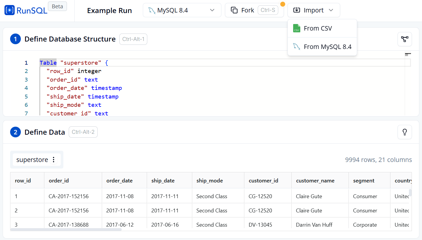
Figure 3. Table creation and data import interface on RunSQL.
-
To practice Pandas queries on Google Colab:
-
Import the Pandas library, read the data, and store it in a DataFrame:
import pandas as pd
data = pd.read_csv('/content/superstore.csv')
df = pd.DataFrame(data)
df.shape   # Output: (9994, 21)
3.3. Exploring and Filtering Data
Query 1: Getting Familiar with the Data
-
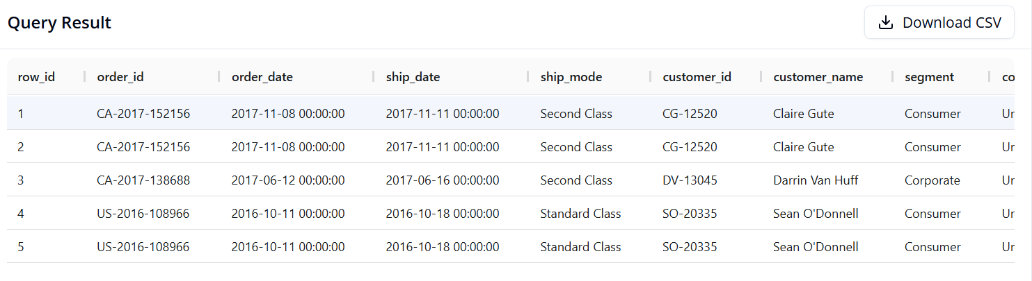
Objective: Display the first 5 rows of data to inspect the table structure.
-
SQL:
SELECT *
FROM superstore
LIMIT 5
- Pandas:
df.head()
- Result:
Query 2: Filtering Data and Selecting Specific Columns
-
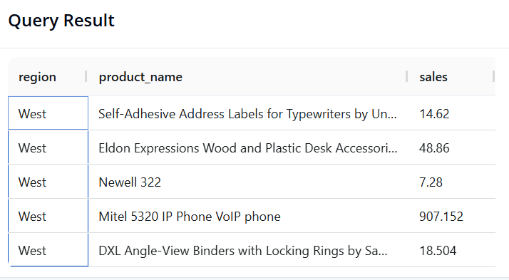
Objective: Preview 5 orders from the West region, showing only the Region, Product Name, and Sales of those orders.
-
SQL:
SELECT region, product_name, sales
FROM superstore
WHERE region = 'West'
LIMIT 5
- Pandas:
result = df.loc[df['region'] == 'West', ['region', 'product_name', 'sales']].head()
- Result:
3.4 Grouping and Aggregation
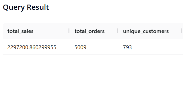
Query 3: Calculating Overall KPIs
-
Objective: Calculate Total Revenue, Total Number of Orders (unique
order_id), and Total Number of Unique Customers across the entire store. -
SQL:
SELECT SUM(sales) AS revenue,
       COUNT(DISTINCT order_id) AS total_orders,
       COUNT(DISTINCT customer_id) AS unique_customers
FROM superstore;
- Pandas:
pd.DataFrame({
    'revenue': [df['sales'].sum()],
    'total_orders': [df['order_id'].nunique()],
    'unique_customers': [df['customer_id'].nunique()]
})
- Result:
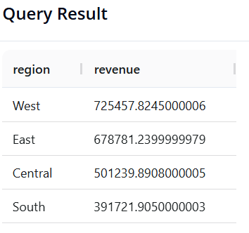
Query 4: Total Revenue by Region
-
Objective: Identify which
regiongenerates the highest sales, sorted from highest to lowest. -
SQL:
SELECT region, SUM(sales) AS revenue
FROM superstore
GROUP BY region
ORDER BY revenue DESC
- Pandas:
(df.groupby('region')['sales']
   .sum()
   .reset_index(name='revenue')
   .sort_values(by='revenue', ascending=False)
)
- Result:
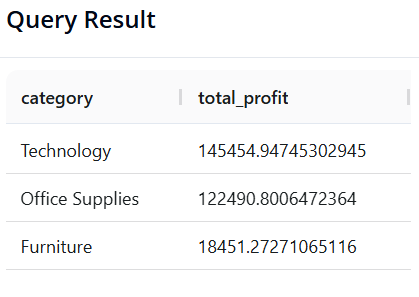
Query 5: Profit by Product Category
-
Objective: Identify which
categorygenerates the most profit. -
SQL:
SELECT category, SUM(profit) AS total_profit
FROM superstore
GROUP BY category
ORDER BY total_profit DESC
- Pandas:
(df.groupby('category')['profit']
   .sum()
   .reset_index(name='total_profit')
   .sort_values(by='total_profit', ascending=False)
)
- Result:
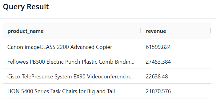
Query 6: Top 5 "Star" Products by Revenue
-
Objective: Find the 5 products (
product_name) with the highest total sales. -
SQL:
SELECT product_name, SUM(sales) AS revenue
FROM superstore
GROUP BY product_name
ORDER BY revenue DESC
LIMIT 5
- Pandas:
(df.groupby('product_name')['sales']
   .sum()
   .reset_index(name='revenue')
   .sort_values(by='revenue', ascending=False)
   .head(5)
)
- Result:
3.5. Multi-Dimensional Analysis and Time Series Processing
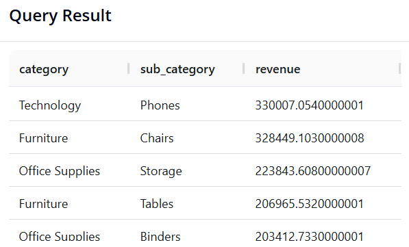
Query 7: Multi-Level Analysis (Category and Sub-Category)
-
Objective: Group by both
categoryandsub_categoryto see which segment generates the highest revenue in detail. -
SQL:
SELECT category, sub_category, SUM(sales) AS revenue
FROM superstore
GROUP BY category, sub_category
ORDER BY revenue DESC
- Pandas:
(df.groupby(['category', 'sub_category'])['sales']
   .sum()
   .reset_index(name='revenue')
   .sort_values(by='revenue', ascending=False)
)
- Result:
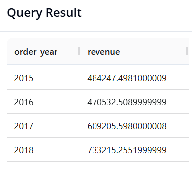
Query 8: Annual Revenue Trend Analysis
-
Objective: Extract the year from the order date column (
order_date) and calculate total revenue per year to observe growth momentum. -
SQL:
SELECT YEAR(order_date) AS order_year, SUM(sales) AS revenue
FROM superstore
GROUP BY order_year
ORDER BY order_year
- Pandas:
# Convert order_date to datetime format first (if not already done)
df['order_date'] = pd.to_datetime(df['order_date'], errors='coerce')

(df.groupby(df['order_date'].dt.year)['sales']
   .sum()
   .reset_index(name='revenue')
)
- Result:
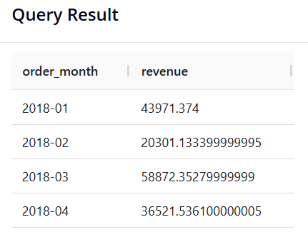
Query 9: Seasonality Analysis (Revenue by Month-Year)
-
Objective: Calculate total revenue broken down by individual month, but limited to data from the year 2018.
-
SQL: We use the
DATE_FORMAT()function to reformat dates into a'Year-Month'string. The%Ysymbol represents the 4-digit year, and%mthe 2-digit month.
SELECT DATE_FORMAT(order_date, '%Y-%m') AS order_month, SUM(sales) AS total_sales
FROM superstore
WHERE YEAR(order_date) = 2018
GROUP BY order_month
ORDER BY order_month
- Pandas:
df['order_date'] = pd.to_datetime(df['order_date'], errors='coerce')

result = (
    df[df['order_date'].dt.year == 2018]
    .assign(order_month=df['order_date'].dt.to_period('M'))
    .groupby('order_month')['sales']
    .sum()
    .reset_index(name='revenue')
)
result
- Result:
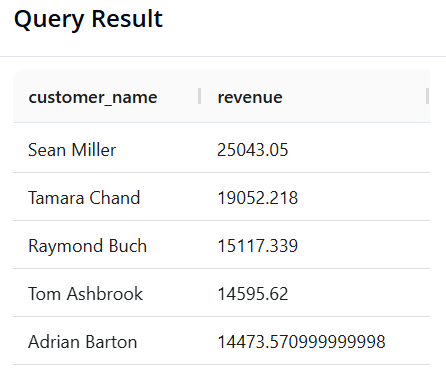
Query 10: Identifying "VIP Customers"
-
Objective: The Marketing team wants to send appreciation gifts to VIP customers. Find the list of customers (
customer_name) whose total lifetime sales (sales) are greater than 14,400, sorted from highest to lowest. -
SQL:
SELECT customer_name, SUM(sales) AS revenue
FROM superstore
GROUP BY customer_name
HAVING revenue > 14400
ORDER BY revenue DESC
- Pandas:
result = (
    df.groupby('customer_name')['sales']
    .sum()
    .reset_index(name='revenue')
    .loc[lambda x: x['revenue'] > 14400]
    .sort_values(by='revenue', ascending=False)
)

result
- Result:
IV. CONCLUSION: SQL OR PANDAS? THE PRACTICAL DECISION
In Sections 2 and 3, you have likely seen that both SQL and Pandas can solve the same analytical problems. This raises the question: "In practice, which tool should we prioritize?"
The answer depends on the following 3 factors.
4.1. Hardware Constraints and Data Size (The Decisive Factor)
-
Pandas (RAM-bound): Pandas loads the entire dataset into the local memory (RAM) of your machine. For a data file of 100MB or 1GB, Pandas handles it very well. However, if you attempt to load a 2-Terabyte (2TB) database, your computer may freeze or throw an out-of-memory error.
-
SQL (Server-powered): SQL databases reside on powerful servers. They are engineered to scan, compute, and filter Terabytes of data (e.g., the entire call history of a large telecommunications company) without needing to download that data to a personal machine.
4.2. Data Storage Source and Format
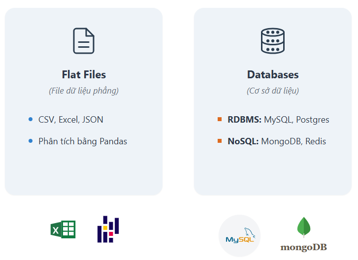
Figure 4. Flat files vs. Databases
-
If the data already resides in a Database Management System, SQL is the best tool for interfacing with it.
-
If the data is provided as flat files (such as
.csv,.excel), or pre-prepared datasets (such as those on Kaggle), Pandas offers an excellent ecosystem for reading and analyzing them immediately.
4.3. Purpose by Stage

Figure 5. The workflow from SQL to Pandas to Machine Learning models. (source: gemini)
-
SQL (Extraction Stage): The primary role is raw filtering and extraction. You use SQL to select only the data relevant to your needs from an enormous "sea" of data.
-
Pandas (Refinement Stage): The primary role is detailed processing. Once you have a smaller dataset in hand, Pandas excels at preprocessing, feature engineering, and preparing data for Machine Learning models.
REFERENCES
-
R. Elmasri and S. B. Navathe, Fundamentals of Database Systems, 7th ed. Hoboken, NJ, USA: Pearson, 2016.
-
The pandas development team, "pandas documentation (Version 1.4)," Feb. 2022. [Online]. Available: https://pandas.pydata.org/pandas-docs/version/1.4/pandas.pdf.
SOURCE CODE
- Link: ⭐ Source Code
Chưa có bình luận nào. Hãy là người đầu tiên!