1. When the Overall View Conceals the Truth

Simpson's Paradox — Two individual data groups show an upward trend, but when combined the trend reverses completely.
Source: AI-generated illustration.
Try a familiar scenario: you're reviewing the results of an A/B test. Variant B wins in every user segment — mobile, desktop, new users, returning users. But when you look at the aggregate numbers, Variant A has a higher overall conversion rate. Which one do you ship?
Or another example: a new drug shows a higher recovery rate than the old drug for both severe and mild patients — but in the combined totals, the old drug looks "more effective." Can that actually happen?
The answer is yes. And this is precisely Simpson's Paradox.
Let's look at concrete numbers to see how this paradox works:
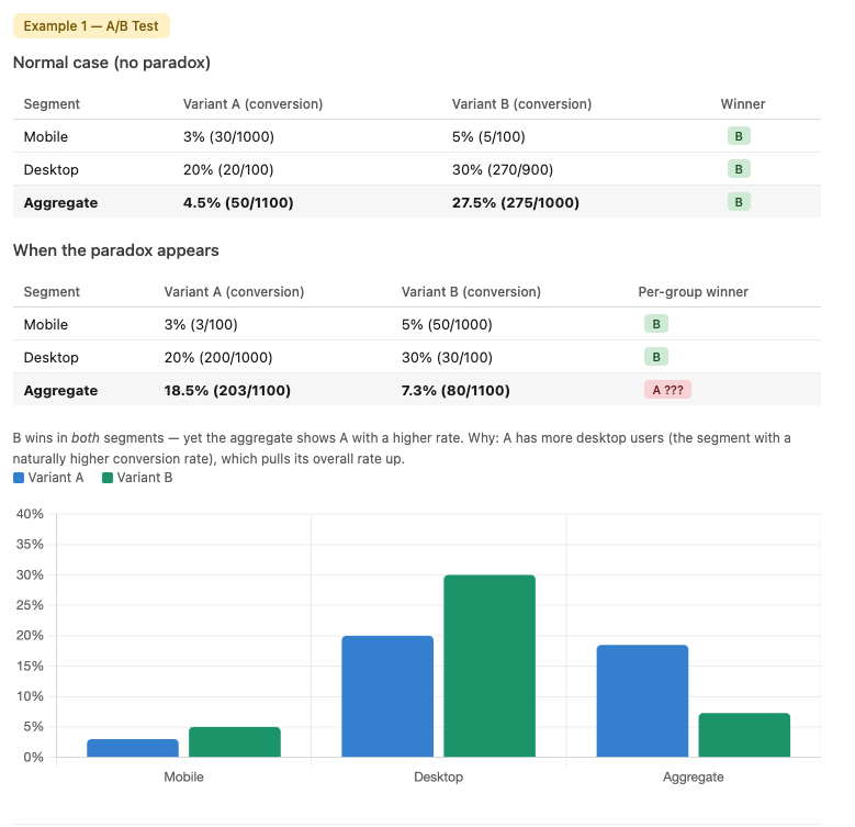
Simpson's Paradox in A/B testing — Variant B wins every segment but loses in the aggregate.
Source: Compiled by the author.
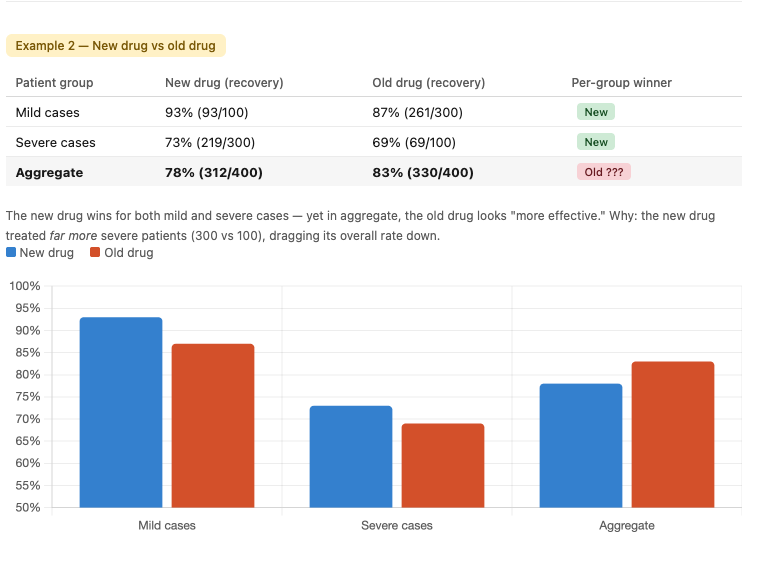
Simpson's Paradox in medicine — the new drug outperforms in each group but loses when data is combined.
Source: Compiled by the author.
What Is Simpson's Paradox?
Simpson's Paradox is a phenomenon in probability and statistics in which a trend that appears in each individual group of data disappears or reverses completely when those groups are combined.
The name "Simpson's Paradox" was introduced by Colin R. Blyth in 1972, although the phenomenon had been described in earlier literature. It is also known as the reversal paradox, the amalgamation paradox, or the Yule–Simpson effect.
Technically, the effect occurs when the marginal association (the relationship between two variables without controlling for other factors) between two categorical variables is qualitatively different from the partial association — that is, the relationship between those two variables after controlling for one or more additional variables.
Simply put: aggregate numbers can lie. When we pool multiple groups of data together, a clear relationship between two variables can reverse or disappear entirely. This is not a calculation error or random noise — it is a direct consequence of hidden structure in the data: lurking variables or imbalances in group sizes are manipulating the overall result without our knowledge.
This is one of the most powerful warnings in data work. So before trusting a rate or a "global" trend, always ask yourself: Is there hidden structure being obscured here?
What This Article Will Cover
In the sections that follow, this article will:
- Explain the mechanism behind the paradox — to understand when it appears and why it is dangerous
- Dissect the classic example of admissions at UC Berkeley — where Simpson's Paradox was once used as evidence in a gender discrimination lawsuit
- Review real-world studies in which the paradox has appeared and led to erroneous conclusions
- Draw practical lessons for anyone working with data
Let's begin by understanding why this paradox exists.
2. The Mechanism of Simpson's Paradox: When Numbers "Deceive" the Eye
Simpson's Paradox is not only a curious phenomenon — it is a costly lesson in interpreting data. It occurs when the relationship between two variables is completely reversed once a third variable is introduced, known as a confounding variable.
Understanding the mechanism behind this paradox not only helps you avoid the trap, but also helps you ask the right questions before drawing any conclusions from data.
2.1. The Rise of Lurking Variables
The core mechanism of this paradox is the shift in weights when data is aggregated. When we only look at aggregated data, we are implicitly assuming that the constituent groups have equivalent structures. But in reality, this is almost never true.
Lurking variables — factors that are uncontrolled or overlooked in the analysis — always exist and quietly distort the true picture.
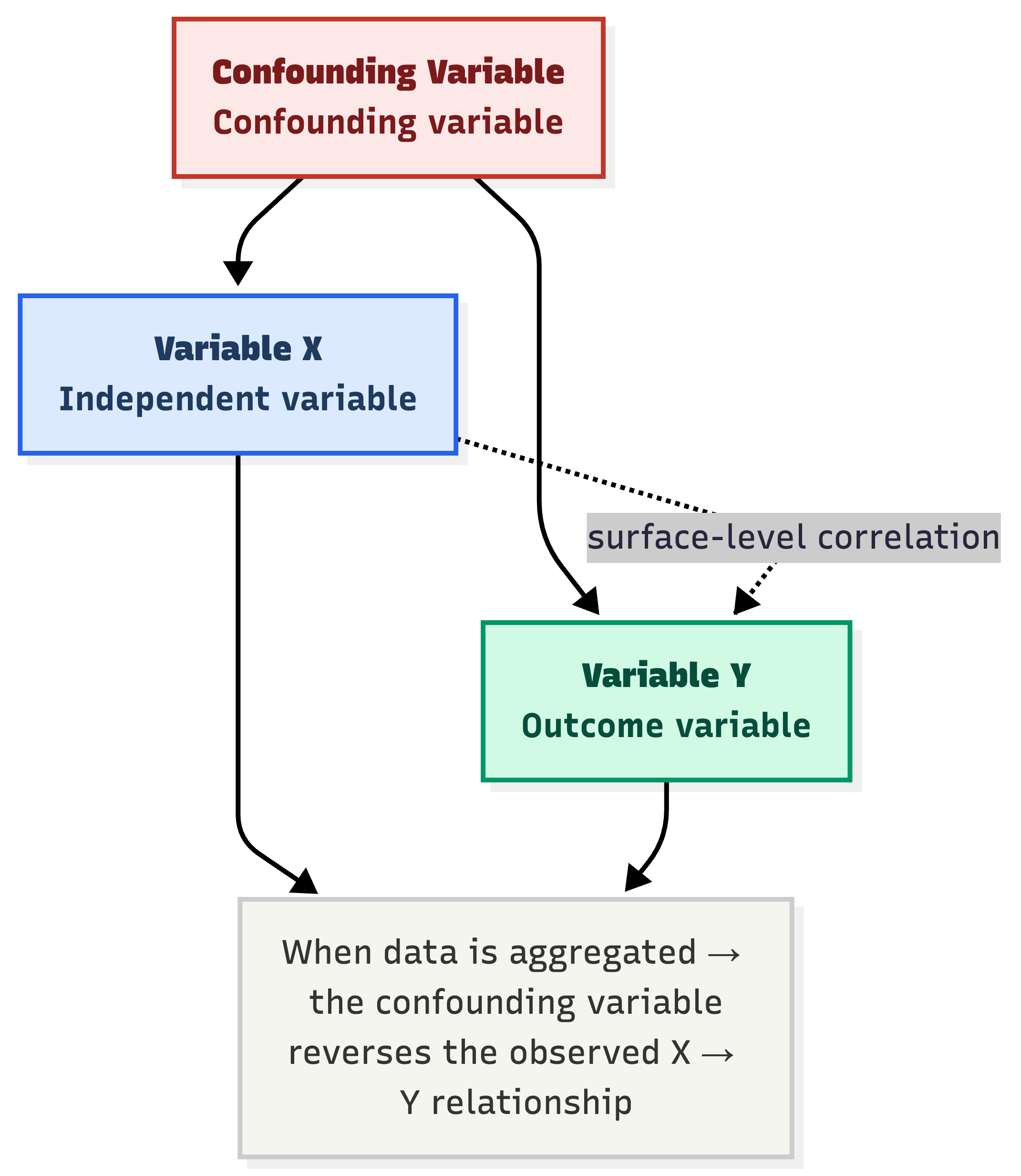
A confounding variable acts on both variable X and variable Y, creating a spurious surface-level correlation when data is pooled.
Source: Compiled by the author.
Mathematically, suppose we compare success rates between methods A and B across two groups:
- Group 1: $P(\text{Success}|A) < P(\text{Success}|B)$
- Group 2: $P(\text{Success}|A) < P(\text{Success}|B)$
But when combined: $P(\text{Success}|A,\ \text{Total}) > P(\text{Success}|B,\ \text{Total})$
This is entirely possible — and it is not a calculation error. It is a direct consequence of unequal sample size distribution across groups.
2.2. Geometric Vector Explanation
One intuitive way to understand this mechanism is through vector representation on a coordinate plane:
- Each group of data is represented as a vector, with the slope corresponding to the success rate ($\text{successes} / \text{total attempts}$).
- When aggregating data, we are performing vector addition of the component vectors.
- Because the lengths (sample sizes) of the vectors differ, the resulting composite vector can have a completely different slope — even pointing in the opposite direction — compared to the individual component vectors.
In other words: whichever group has the larger sample will "pull" the aggregate vector toward itself more forcefully, regardless of that group's actual effectiveness.
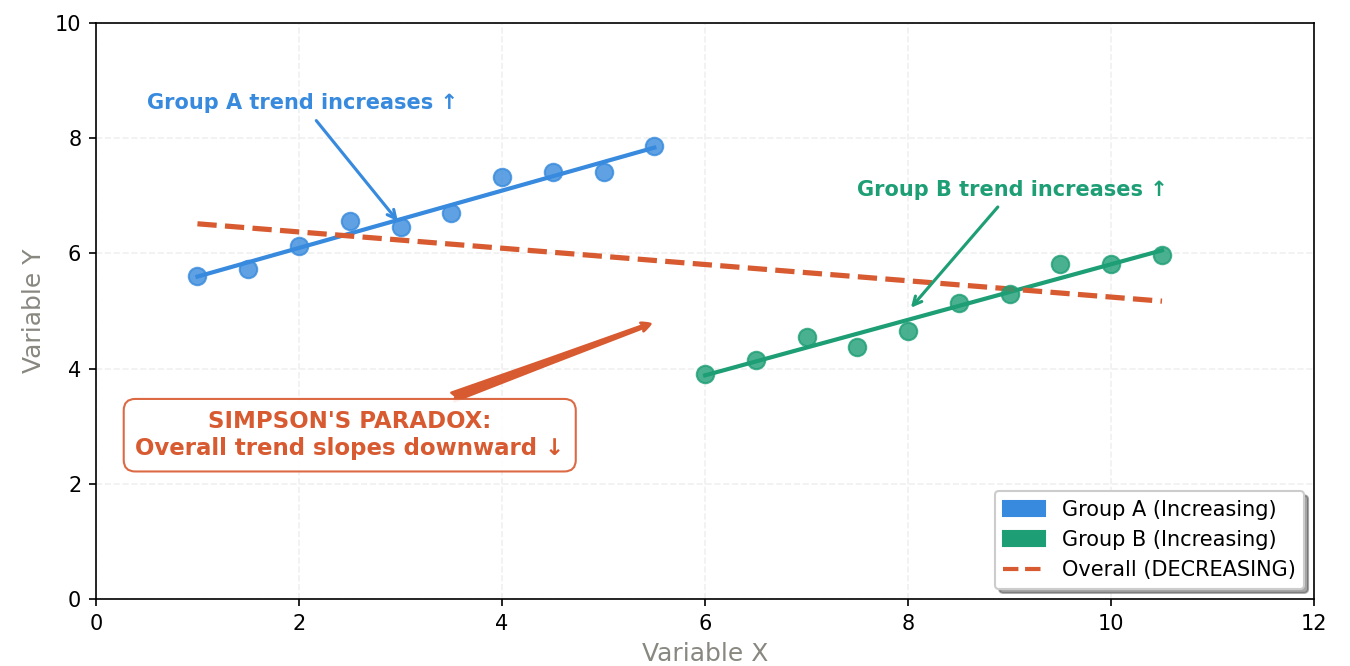
Group A (blue) and Group B (green) both show upward trends individually — but the combined trend line (red, dashed) reverses downward because the two groups occupy different value ranges.
Source: Compiled by the author.
2.3. The Effect of Sample Size and "Toxic Weighting"
The paradox typically emerges when sample size is inversely proportional to effectiveness — meaning the group with the larger sample has worse outcomes, and vice versa:
Case 1 — Large sample, low effectiveness: A group with an enormous number of observations but poor results will pull down the overall average, obscuring the successes in smaller groups.
Case 2 — Small sample, high effectiveness: Strong results within a small group are often "swallowed up" when placed alongside much larger groups.
This is precisely why percentages alone are never sufficient — you need to know how many observations that figure is based on, and whether the groups are proportionally balanced.
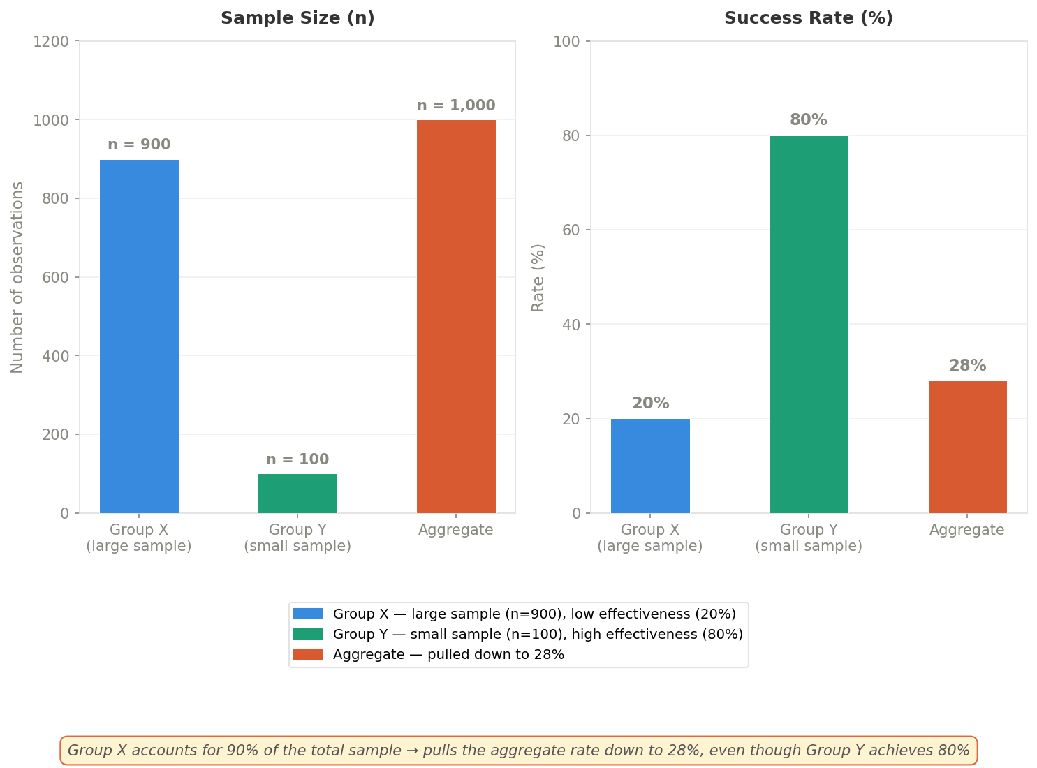
Group X (n=900, 20% rate) dominates in sample size, pulling the aggregate rate down to 28% — even though Group Y achieves 80%.
Source: Compiled by the author.
2.4. The Danger in Observational Research
Simpson's Paradox is especially dangerous in observational studies — that is, studies without random assignment. In these cases, subjects self-select into their groups, leading to systematic differences between groups that we cannot control.
The real-world consequences are alarming:
- Policy mistakes: A manager might discard a genuinely good option — one that performs well across every segment — simply because the aggregate number looks worse.
- Medical risks: A drug might help every group of patients, but if aggregate data shows it performing worse than a placebo (because sicker patients received the new drug more often than milder cases), it could be unjustly removed from treatment protocols.
How to guard against it:
- Stratify the data: Always break down data by characteristic variables before drawing conclusions — age, gender, severity, or any variable that could influence the outcome.
- Visualize by group: Draw scatter plots or bar charts for each group before aggregating — many paradoxes will reveal themselves at this step.
- Check the weights: Always ask: "Are the sample sizes across groups highly unequal? Which group is carrying the most weight in the total?"
Simpson's Paradox is a reminder that data analysis is not just calculation — it is also about asking the right questions before trusting any number.
3. The Classic Example — UC Berkeley
If Simpson's Paradox needed a "living proof" to enter textbooks, the 1973 admissions story at the University of California, Berkeley would be the perfect candidate.
3.1. Background
In the fall of 1973, the Graduate Division of the University of California, Berkeley published statistics on all applications to the university's graduate programs. The initial goal was clear: to examine whether there was gender bias in the admissions process — an issue of significant legal and ethical importance given the social context of the time.
The results were startling.
3.2. Diving Into the Data
Looking at the aggregate data across the entire university, the numbers appeared unmistakable:
| Applications | Admission Rate | |
|---|---|---|
| Men | 8,442 | 44% |
| Women | 4,321 | 35% |
| Total | 12,763 | — |
A 9-percentage-point gap — and chi-square tests confirmed the probability of this difference occurring by chance was extremely low. Every sign pointed to a single conclusion: Berkeley was discriminating against women.
But the story did not end there.
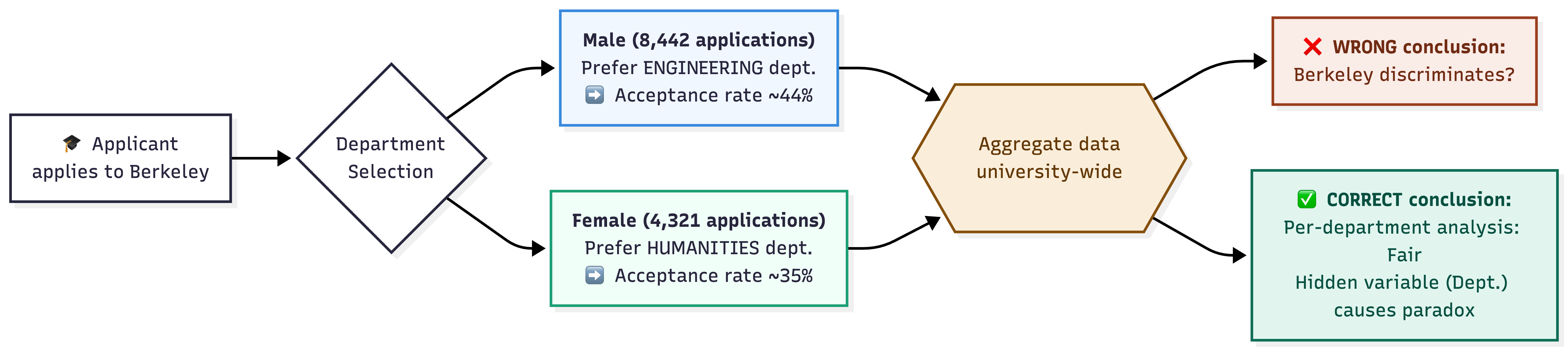
The full causal chain leading to Simpson's Paradox in Berkeley admissions — the aggregate view yields the wrong conclusion; separating by department reveals the truth.
Source: Compiled by the author.
3.3. Decoding the Paradox
When researchers began breaking down the data by department, the picture changed completely.
When examining each department individually — particularly the six largest — the apparent bias favoring men vanished entirely. In fact, in some departments the data even showed a slight preference for female applicants.
So what had happened?
The true cause lay in a variable that had been entirely overlooked in the initial analysis: the applicants' choice of department.
- Women tended to apply to departments with highly competitive, difficult admissions — such as the humanities — where acceptance rates were low for both genders.
- Men, conversely, tended to apply to departments with higher acceptance rates — such as engineering.
The result: even though each individual department operated completely fairly, the overall female admission rate was lower than the overall male rate — simply because the two groups were competing on two entirely different playing fields.
3.4. Conclusions from This Example
The study published in Science in 1975 (Bickel, Hammel & O'Connell) drew two important conclusions:
On the admissions process: There was no evidence of systematic discrimination from departmental admissions committees. The process was conducted fairly — the disparity in aggregate data reflected deeper social and educational factors that caused men and women to gravitate toward different fields of study.
Statistically: This became the canonical example of Simpson's Paradox, illustrating that aggregating data from groups with different characteristics — here, departments with different levels of competitiveness — can lead to conclusions completely opposite to the reality within each individual group.
Core lesson: When analyzing data about fairness, looking at aggregate figures is not enough. We must examine the intermediate variables — such as choice of field of study — to correctly understand the true causal relationship underlying the data.
4. Simpson's Paradox Through the Lens of Modern Research
The UC Berkeley story happened more than 50 years ago — but Simpson's Paradox has not become obsolete. In the era of Big Data and AI, as data volumes grow exponentially, the risk of being "deceived" by this paradox is greater than ever. Below are several recent studies showing that the paradox is still present — and growing more complex.
4.1. Machine Learning and Algorithmic Fairness
One of the most concerning applications of Simpson's Paradox is in the field of algorithmic fairness — the question of whether AI models treat all groups of people equitably.
A 2025 study by Babaei et al. posed the problem in the context of credit lending in New York: an AI model might look entirely fair when analyzed in aggregate, but conceal discriminatory treatment when examining individual demographic groups. Simpson's Paradox is the very mechanism hiding that injustice.
To detect these hidden biases, the authors proposed using Shapley values — a method for measuring the degree of influence each variable has on a model's decision. Their findings showed that looking only at a model's overall accuracy is insufficient — only by disaggregating by subgroup does the true picture emerge.
4.2. Simpson's Paradox in Social Data
Simpson's Paradox also appears in less expected places — such as in analyzing public opinion reactions on social media.
Liu and Son (2025) analyzed the relationship between COVID-19 severity and news coverage and social media opinions in China during 2020–2022. When looking at the full three years combined, the data showed a surprising negative correlation: the worse the outbreak, the less news response it generated.
However, when the data was split by individual year, the results reversed completely — a clear positive correlation emerged: rising case counts led to increased news coverage. The study concluded that pooling multi-period data can conceal the true psychological and emotional responses of public opinion at specific moments in time — an important warning for anyone analyzing time-series data.
4.3. Beyond the Concept of "Confounding Variables"
For many years, leading causal inference researcher Judea Pearl argued that Simpson's Paradox is fundamentally a consequence of confounding variables — and that controlling for those variables is what resolves the paradox.
But a 2024 study by Dong et al. challenged this view. The authors showed that the paradox can arise from a variety of causes, not always related to causality — for example, random variation in evolutionary biological data, or simply the incorrect definition of boundaries between groups when aggregating data.
Along a different line, Sarkar and Bandyopadhyay (2021) emphasized that to truly resolve Simpson's Paradox in practice, one cannot rely on a single tool. It requires a combination of causal reasoning, statistical methods, and contextual judgment — because sometimes the paradox has no single "correct" answer; it depends on the question you are actually trying to answer.
Overall, modern research suggests that Simpson's Paradox is not merely a statistical problem to be "fixed" — it is a fundamental reminder: data does not speak the truth on its own; it is the analyst who decides which questions need to be asked.
5. Conclusions and Lessons
From the Berkeley admissions story in 1973 to AI credit-lending models in 2025 — Simpson's Paradox has traveled a long road, but its core message has not changed: aggregate numbers can hide the truth, and sometimes they hide it perfectly.
5.1. What the Paradox Has Taught Us
Simpson's Paradox is both a demonstration and a profound warning: statistical data is not always absolute truth in the absence of context. Data itself does not "know how to lie" — it is the way we group, oversimplify, and superficially interpret it that inadvertently obscures the true nature of the problem.
This phenomenon reveals the danger of blindly trusting averages or aggregate ratios. When we ignore hidden factors or disparities in group sizes, we easily fall into cognitive traps — leading to flawed assessments with significant real-world consequences, whether in admissions policy, medical treatment protocols, or business strategy.
Looking back across the entire article, there are four key lessons that anyone working with data should internalize:
Always be skeptical of "aggregate figures." Never be satisfied with the big picture. When faced with an average rate or a combined result, develop the habit of asking: "Is there any grouping factor — such as age, gender, region, or product segment — that could completely change the picture if we break the data down?"
Hunt for confounding variables. The overall picture is often distorted by a third factor not yet accounted for — like the difficulty level of different departments in the UC Berkeley story. Decomposing data into small, internally homogeneous groups is a mandatory step toward uncovering the truth.
Understand the context in which the data was generated. Technical proficiency alone is not enough. A data practitioner needs to understand the story behind the data: how was it collected? Was the sample allocation random and balanced? Context is the key to decoding statistical paradoxes.
Exercise caution when inferring causality. Simpson's Paradox reminds us that a correlation at the aggregate level can reverse completely at the detailed level. We must be extremely careful about using observational data to assert that factor A is a direct cause of outcome B.
5.2. A Practical Checklist for Data Practitioners
The next time you look at an aggregate figure — whether it is an A/B test result, a performance report, or medical statistics — ask yourself:
1. Has the data been stratified?
Break it down by key characteristic variables (age, gender, region, product segment, etc.) before drawing conclusions.2. Are the group sample sizes highly unequal?
Which group carries the most weight? Is it pulling the overall result toward itself?3. Are there uncontrolled variables?
Did subjects self-select into their groups? If so, what factors influenced that selection?4. Are the aggregate trend and the within-group trends consistent?
If not — that is a signal to investigate further, not to ignore.
5.3. Closing Thoughts
Simpson's Paradox is one of the reasons why data analysis is both a science and an art. Statistical tools are growing ever more powerful, and data volumes ever larger — but the risk of being misled by aggregate figures does not diminish as a result.

The truth does not lie in the overall picture — it hides within each individual piece of the puzzle.
Source: AI-generated illustration.
Understanding this paradox does not mean you will never make a mistake. But it equips you with an important habit: always question a number before believing it — no matter how obvious it appears.
Because sometimes, the truth does not lie in the big picture — it hides in each small piece of the puzzle that you have not yet looked closely at.
References
Babaei, G., Giudici, P., & Neelakantan, P. (2025). Explainability, fairness and the Simpson's paradox in credit lending. Physica A: Statistical Mechanics and its Applications, 680, 131030. https://doi.org/10.1016/j.physa.2025.131030
Bickel, P. J., Hammel, E. A., & O'Connell, J. W. (1975). Sex bias in graduate admissions: Data from Berkeley. Science, 187(4175), 398–404. https://doi.org/10.1126/science.187.4175.398
Blyth, C. R. (1972). On Simpson's paradox and the sure-thing principle. Journal of the American Statistical Association, 67(338), 364–366. https://doi.org/10.2307/2284382
Dong, Z., Cai, W., & Zhao, S. (2024). Simpson's paradox beyond confounding. European Journal for Philosophy of Science, 14(44). https://doi.org/10.1007/s13194-024-00610-8
Kievit, R. A., Frankenhuis, W. E., Waldorp, L. J., & Borsboom, D. (2013). Simpson's paradox in psychological science: A practical guide. Frontiers in Psychology, 4, 513. https://doi.org/10.3389/fpsyg.2013.00513
Liu, Q., & Son, H. (2025). Simpson's paradox of social media opinion's response to COVID-19. Frontiers in Public Health, 13, 1448811. https://doi.org/10.3389/fpubh.2025.1448811
Sarkar, P., & Bandyopadhyay, P. S. (2021). Simpson's paradox: A singularity of statistical and inductive inference. arXiv preprint arXiv:2103.16860v2. https://arxiv.org/abs/2103.16860
Simpson, E. H. (1951). The interpretation of interaction in contingency tables. Journal of the Royal Statistical Society, Series B, 13(2), 238–241. https://doi.org/10.1111/j.2517-6161.1951.tb00088.x
Chưa có bình luận nào. Hãy là người đầu tiên!