Overview

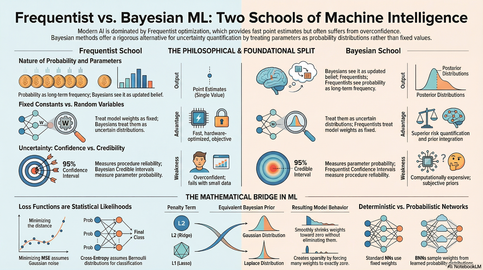
The explosion of AI and Machine Learning, particularly Deep Learning, has completely reshaped humanity's computing and problem-solving capabilities. This capability is largely built upon point estimation methods belonging to the Frequentist school of thought. Algorithms such as Stochastic Gradient Descent (SGD) or Adam yield outstanding performance in tasks like image recognition, natural language processing, and recommendation systems. However, this success comes with a systemic drawback: traditional Deep Learning models are often overconfident in their predictions, even when facing completely unfamiliar data or out-of-distribution data. This poses catastrophic risks in safety-critical systems such as medical diagnosis, autonomous driving, or financial risk analysis, where a wrong prediction can lead to severe consequences for life and property. In this context, the rise of uncertainty quantification methods based on Bayesian statistics becomes the solution to the problem. Bayesian Neural Networks (BNNs) emerge as a compromise between the representational power of Deep Learning and the rigor in probabilistic reasoning of Bayesian mathematics.
The core difference in the performance and decision-making mechanisms of Machine Learning models does not simply lie in the network architecture or datasets, but stems from profound contradictions in the fundamental philosophy regarding the concept of "probability". The Frequentist school defines probability as the long-run frequency of an event, whereas the Bayesian school defines probability as a subjective degree of belief that is continuously updated through data.
This philosophical divergence leads to Machine Learning algorithms that operate in entirely different ways, especially when confronted with two extremes of data: massive data and small, noisy data. While Frequentist models often collapse or yield misleading conclusions when the sample size is small due to the violation of asymptotic assumptions, Bayesian methods exhibit superior strength thanks to their ability to integrate prior knowledge. The question is how to map this philosophical difference into the specific mathematical formulas that constitute modern Machine Learning models, and accurately measure the trade-offs between them in an experimental setting.

The objectives of the study include:

• Dissecting the mathematical and philosophical foundations of each school, clarifying how they define parameters and data.
• Analytically proving the equivalence between core Machine Learning concepts (such as MSE and Cross-Entropy loss functions, and $L_1$/$L_2$ Regularization techniques) and statistical estimation methods (MLE, MAP).
• Establishing a rigorous experimental design to compare the performance, calibration capability, and uncertainty quantification of the two schools.
• Analyzing the trade-offs in computational cost and interpretability, thereby providing practical recommendations for deployment in industrial environments.

1. Mathematical Foundations

Analyzing Statistical Machine Learning requires a clear distinction in how different schools of thought perceive two core entities: model parameters (denoted as $\theta$) and observed data (denoted as $X$ or $D$). This distinction shapes all the accompanying inference tools and optimization algorithms.

1.1. The Frequentist Paradigm

From the Frequentist perspective, probability is strictly objective and is tied to the repetition of events within a sample space, or the relative frequency of that event as the number of trials approaches infinity. Based on this philosophy, model parameters $\theta$ are defined as fixed but unknown constants existing in nature. Frequentism does not assign any probability distribution to $\theta$. Conversely, the data $X$ is considered a random variable generated by a data-generating mechanism governed by $\theta$.

1.1.1. Maximum Likelihood Estimation (MLE)

The sharpest and most fundamental tool of the Frequentist school is Maximum Likelihood Estimation (MLE). Since $\theta$ is a constant, the goal of inference is not to find the "probability of $\theta$" (a meaningless concept in Frequentism), but rather to find the value of $\theta$ that makes the observed data $X$ most probable.
The Likelihood function $L(\theta|X)=P(X|\theta)$ measures the goodness-of-fit of the model to the data. MLE seeks a point estimate $\hat{\theta}_{MLE}$ such that$$\hat{\theta}_{MLE}=\arg\max_{\theta} P(X|\theta)$$To facilitate analytical computation and avoid numerical underflow when multiplying the very small probabilities of independent samples, the natural logarithm is often applied, creating the Log-Likelihood function:$$\hat{\theta}_{MLE} = \arg\max_{\theta}\sum_{i=1}^N \log P(x_i|\theta)$$MLE provides a single point estimate that is completely data-driven and unaffected by any external subjective beliefs or assumptions. This provides objectivity, but simultaneously makes the model susceptible to being misled by noise if the sample size is too small.

1.1.2. Confidence Intervals and Hypothesis Testing (p-value)

Because the uncertainty of $\theta$ cannot be represented by a probability distribution, Frequentists use Confidence Intervals (CIs) and p-values to quantify the uncertainty of the statistical procedures themselves. A classic mistake in data science is interpreting a "$95\%$ Confidence Interval" as meaning "there is a $95\%$ probability that the true parameter $\theta$ lies within this interval". From the Frequentist perspective, $\theta$ is a constant, therefore it either lies within the interval or it does not (1 or 0). The true meaning of CIs is: If we repeat the sampling process and construct this confidence interval an infinite number of times, $95\%$ of the generated intervals will contain the true constant $\theta$. Similarly, the p-value is not the probability that the null hypothesis is true, but rather the probability of observing data as extreme as or more extreme than the current data, assuming that the null hypothesis is true. This complex and convoluted interpretation often leads to misuse and the reproducibility crisis in research.

1.2. The Bayesian Paradigm

The Bayesian paradigm builds a completely inverted worldview. Probability is no longer bound to the frequency of repetition, but is expanded into a logical system to represent a reasonable "degree of belief" about a state of the world. In this framework, the observed data $X$ is a fixed truth; conversely, the model parameters $\theta$ are unobservable and uncertain quantities, and therefore they must be modeled as random variables with their own probability distributions. This allows researchers to directly integrate expert knowledge, historical information, or skepticism into the model prior to observing any data.

1.2.1. Bayes' Theorem and the Belief Updating Mechanism

The heart of the Bayesian method is a learning mechanism based on updating information via Bayes' Theorem, a mathematical elegance that connects past beliefs with current evidence:$$P(\theta|X) = \frac{P(X|\theta)P(\theta)}{P(X)}$$Where:
- Prior Distribution (Prior - $P(\theta)$): Represents the initial belief or assumption about the parameter $\theta$ before seeing the data $X$. Choosing a Prior is an art and also the biggest source of controversy (due to its subjectivity).
- Likelihood Function (Likelihood - $P(X|\theta)$): Represents the degree to which the data $X$ supports specific values of $\theta$. This is the exact component shared with the Frequentist method.
- Posterior Distribution (Posterior - $P(\theta|X)$): This is the ultimate result of the Bayesian inference process. It represents the updated belief about $\theta$ after taking the observed data into account.
- Marginal Likelihood / Evidence ($P(X)$): The total probability of the data, calculated by the integral $\int P(X|\theta)P(\theta)d\theta$. Although it acts as a normalizing constant to ensure the Posterior is a valid probability distribution, computing this integral for high-dimensional parameter spaces (such as in Deep Learning) is highly intractable, leading to the emergence of complex approximation methods.

1.2.2. MAP Estimation and Fully Bayesian Inference

Since manipulating the entire Posterior distribution often exceeds computational limits, a pragmatic intermediate step commonly used is Maximum A Posteriori (MAP) Estimation. MAP does not retain the entire distribution, but only seeks a single point that maximizes the Posterior:$$\theta_{MAP} = \arg \max_{\theta} [P(X|\theta)P(\theta)]$$Moving to the logarithmic space:$$\theta_{MAP} = \arg\max_{\theta}[\log P(X|\theta) + \log P(\theta)]$$ It can be clearly seen that MAP is an extension of MLE, being "pulled" or "regularized" by the presence of $\log P(\theta)$.
However, MAP remains merely a point estimate with a Frequentist undertone. The Fully Bayesian Inference method refuses to reduce this information. Instead of returning a single optimal parameter, it retains the full Posterior distribution $P(\theta|X)$ and computes the prediction for a new data point x^* by integrating over the entire parameter space:$$P(y^*|x^*,X) = \int P(y^*|x^*, \theta)P(\theta|X)d\theta$$This is precisely the Predictive distribution, which directly represents the risks and uncertainty of the model.

1.2.3. Credible Intervals

Thanks to the distributional nature of $\theta$, Bayesian provides Credible Intervals. In stark contrast to Confidence Intervals, a $95\%$ Credible Interval has an extremely intuitive interpretation that aligns with human intuition: "Based on the observed data and prior belief, there is a $95\%$ probability that the true parameter actually lies within this interval". The ability to make direct probabilistic statements is one of the biggest driving forces leading data scientists to shift towards Bayesian approaches in business risk analysis and medical applications.

2. Equivalence and Differences in Machine Learning

2.1. Loss Functions from a Statistical Perspective

In Machine Learning model training, Loss Functions are not chosen based on intuitive experience, but are the inevitable analytical consequences of the Maximum Likelihood Estimation (MLE) method under different assumptions about the distribution of noise in the data.

2.1.1. Mean Squared Error (MSE) is MLE with Gaussian noise

We begin with a pivotal assumption: the error between the true label $y^{(i)}$ and the model's prediction $\hat{y}^{(i)} = f(x^{(i)};\theta)$ follows a Normal (Gaussian) distribution with a mean of 0 and variance $\sigma^2$. In other words, $y^{(i)}$ is sampled from a conditional distribution: $P(y^{(i)}|x^{(i)};\theta) = \mathcal{N}(\hat{y}^{(i)}, \sigma^2)$.
The Probability Density Function (PDF) of the Gaussian distribution for a single data point is:$$P(y^{(i)}|x^{(i)};\theta) = \frac{1}{\sqrt{2\pi\sigma^2}} \exp\left(-\frac{(y^{(i)} - \hat{y}^{(i)})^2}{2\sigma^2}\right)$$For a dataset comprising independent observations, the conditional Log-Likelihood function is the sum of the logarithms of each individual PDF:$$\log L(\theta) = \sum_{i=1}^{N}\log\left(\frac{1}{\sqrt{2\pi\sigma^2}} \exp \left(-\frac{(y^{(i)} - \hat y^{(i)})^2}{2\sigma^2}\right)\right)$$Applying basic logarithmic properties to expand the expression:$$\log L(\theta) = \sum_{i=1}^{m} \left[\log\left(\frac{1}{\sqrt{2\pi\sigma^2}}\right) - \frac{(y^{(i)} - \hat y^{(i)})^2}{2\sigma^2}\right]$$$$=-m\log(\sqrt{2\pi\sigma^2}) - \frac{1}{2\sigma^2}\sum_{i=1}^m\left(y^{(i)}-\hat y^{(i)}\right)^2$$The MLE method requires us to find $\theta$ to maximize $\log L(\theta)$. Note that the first term $-m\log(\sqrt{2\pi\sigma^2})$ and the multiplicative constant $\frac{1}{2\sigma^2}$ are completely independent of the model's weights $\theta$. Therefore, finding the maximum of $\log L(\theta)$ is entirely equivalent to finding the minimum of the residual term containing $\theta$:$$\theta_{MLE} = \arg \min_\theta \sum_{i=1}^m (y^{(i)}-\hat y^{(i)})^2$$When dividing this expression by the constant $m$ for normalization, we obtain the exact mathematical definition of Mean Squared Error (MSE). This elegantly proves that: Attempting to minimize MSE is essentially seeking the parameters most likely to generate the observed data, under the assumption that the natural world is corrupted by random fluctuations following a Normal distribution.

2.1.2. Cross-Entropy Loss is MLE for Categorical/Bernoulli distribution

Moving to Classification problems, the label $y$ is no longer a continuous value with Gaussian noise, but rather a discrete variable. For binary classification, $y\in\{0,1\}$. This data generation process is most accurately described by the Bernoulli distribution.
Suppose the neural network outputs the probability $\hat y^{(i)} = P(y^{(i)}=1|x^{(i)};\theta)$. The probability of the actual class $y^{(i)}$ occurring is combined into a single Bernoulli equation:$$P(y^{(i)}|x^{(i)};\theta) = \sum_{i=1}^{m} \log[(\hat y^{(i)})^{y^{(i)}}(1-\hat y^{(i)})^{(1-y^{(i)})}]$$Using the property $\log(a^b)=b\log a$, we bring the exponent down:$$\log L(\theta) = \sum_{i=1}^m [y^{(i)}\log(\hat y^{(i)}) + (1-y^{(i)})\log(1 - \hat y^{(i)})]$$This is the immutable mathematical prototype of the Binary Cross-Entropy function. Expanded to multi-class problems, the Bernoulli distribution becomes a Categorical (Multinomial) distribution, and a similar corollary leads to the Categorical Cross-Entropy function. Thus, the term "Cross-Entropy" originates from Information Theory, but is essentially a "misnomer" for maximizing the Likelihood function within the Statistical reference frame.

2.2. Regularization is Bayesian Priors

If MLE maps directly to base loss functions, then MAP Estimation is the mathematical backbone of Regularization techniques aimed at combating overfitting. $L_1$ and $L_2$ Regularization are not arbitrary inventions; they carry a completely transparent Bayesian Probabilistic interpretation: adding penalty terms is equivalent to imposing specific Prior Distributions on the model's weights.
Recalling the MAP equation, the objective is to maximize: $\log P(D|\mathbf{w}) + \log P(\mathbf{w})$. Converting to minimizing the loss function, we have:$$Loss(\mathbf{w}) = -\log P(D|\mathbf{w}) - \log P(\mathbf{w})$$The component $-\log P(D|\mathbf{w})$ is exactly MSE or Cross-Entropy. The second component, $-\log P(\mathbf{w})$, is precisely the Regularization algorithm.

2.2.1. $L_2$ Regularization (Ridge) is equivalent to Gaussian Prior

Suppose we have a subjective Bayesian belief that the weights $\mathbf{w}$ should not be too large, and they fluctuate around $0$ according to a Normal (Gaussian) distribution with variance $\tau^2$. The PDF of this Gaussian Prior is: $P(\mathbf{w}) = \prod_j\frac{1}{\sqrt{2\pi\tau^2}} \exp \left( -\frac{w_j^2}{2\tau^2} \right)$. When we take $-\log P(\mathbf{w})$, the constants are discarded, the exponent is brought down and the negative sign is canceled out:$$-\log P(\mathbf{w}) \propto \sum_j \frac{w_j^2}{2\tau^2} = \frac{1}{2\tau^2} ||\mathbf{w}||_2^2$$Letting $\lambda=\frac{1}{2\tau^2}$, we obtain exactly the penalty term of $L_2$ Regularization: $\lambda||\mathbf{w}||_2^2$.
Geometric & practical meaning: The Gaussian distribution has a smooth, gentler curve around $0$. Therefore, $L_2$ heavily penalizes extremely large weights but is "lenient" towards small weights, resulting in the weights being shrunk down but very rarely forced to absolute $0$. It creates circular constraint spaces ensuring strict convexity for the objective function.

2.2.2. $L_1$ Regularization (Lasso) is equivalent to Laplace Prior

Instead of penalizing with squares, $L_1$ Regularization penalizes with absolute values. The mathematical magic happens when we impose a Laplace distribution as the Prior. The PDF of the Laplace distribution with a mean of $0$ and a scale parameter $b$ is: $P(\mathbf{w}) = \prod_j \frac{1}{2b} \exp \left( -\frac{|w_j|}{b} \right)$. Applying the transformation $-\log P(\mathbf{w})$, we have:$$-\log P(\mathbf{w}) \propto \sum_j \frac{|w_j|}{b} = \frac{1}{b} ||\mathbf{w}||_1$$Letting $\lambda = \frac{1}{b}$, we obtain exactly the $L_1$ penalty: $\lambda||\mathbf{w}||_1$.
Geometric & practical meaning: Contrary to Gaussian, the Laplace distribution possesses a sharp peak exactly at $0$ and heavy tails. This sharp peak reflects an extremely strong Bayesian belief that the majority of weights should truly be zero (sparsity), while the heavy tails allow a very few weights with large values to exist. Geometrically, $L_1$ creates diamond-shaped constraint regions with sharp corners lying on the coordinate axes, causing the optimal solution to frequently intersect right at these corners (where some variables are completely eliminated), making $L_1$ an excellent Feature Selection technique.
This proof affirms: The use of $L_1$/$L_2$ Regularization, although possibly considered part of the Frequentist school, is essentially implicitly executing Bayesian approaches unconsciously.

2.3. Model Architecture Comparison: Traditional Neural Networks vs. Bayesian Neural Networks (BNNs)

The most distinct divergence between the two schools is exposed in how they construct the architecture of Neural Networks.

2.3.1. Traditional Neural Networks (Frequentist)

Traditional deep neural networks (DNNs) operate as a deterministic mapping mechanism. The training process uses SGD and Backpropagation to traverse the entire optimization space to find a single optimal set of weights $\mathbf{w}$ (MLE or MAP) that minimizes the loss function. Consequently, the model generates only a single decision boundary. When asked to predict on new data $x^*$, it outputs a single value (e.g., "The probability of the patient having cancer is $99\%$"). This structure does not carry any inherent concept of its own skepticism, leading to a fatal weakness: The model still returns a $99\%$ confidence even when the input data is random white noise or out-of-distribution data, rendering it completely fragile against adversarial attacks.

2.3.2. Bayesian Neural Networks (BNNs)

The architecture of BNNs (Bayesian Neural Networks) rejects assigning a constant value to each neuron connection. Instead, each weight and bias is replaced by a probability distribution (usually a learnable Normal distribution with parameters $\mu$ and $\sigma$). Training BNNs is the process of updating the shape of millions of these distributions via Bayes' Theorem (from Prior to Posterior $p(\mathbf{W}|D)$).
This structure creates a profound difference in the Inference mechanism: BNNs do not produce a static prediction. Each time a prediction is made, the network samples a random set of weights from its Posterior distribution. Performing this hundreds of times through Monte Carlo integration, the network generates a distribution of predictive outcomes rather than a single point.
If all sampling iterations yield the same result (e.g., "The patient is healthy"), the model doesn't just say "I think the patient is healthy", but also indicates "I am extremely certain about this decision" (low Uncertainty).
If the samples produce strongly contradictory results (e.g., spanning from $10\%$ to $90\%$), the model signals: "I don't know, this data is beyond my understanding" (high Epistemic Uncertainty). Thanks to the ability to "know what it doesn't know" (aware of its own limitations), BNNs become an invaluable safety barrier in systems that demand rigorous risk management.

3. Experimental Design

3.1. Evaluation Metrics

The transition from MLE to BNNs requires an upgraded set of evaluation metrics. Relying solely on RMSE (for regression) or Accuracy (for classification) is completely inadequate because they are point-estimate metrics, completely blind to the model's uncertainty.
To address this issue, Uncertainty Metrics were introduced to evaluate whether a model is trustworthy or not:

3.1.1. Expected Calibration Error (ECE)

ECE is the most popular intuitive metric for evaluating the calibration of predictions, i.e., whether the model's confidence matches the actual probability.
The algorithm partitions the confidence space into $M$ equally sized bins. Within each bin, it compares the average Confidence with the actual observed Accuracy of the data points falling into that bin. The formula calculates the weighted average of the absolute difference in each bin:$$\text{ECE} = \sum_{m=1}^{M} \frac{|B_m|}{n} | \text{acc}(B_m) - \text{conf}(B_m) |$$Despite its popularity, ECE faces severe criticism from the Bayesian academic community. Its biggest drawback is its heavy reliance on the number of bins chosen. More seriously, a completely passive model (which only predicts based on class priors, without learning any knowledge) can still achieve a perfect ECE of 0 if the data is uniformly distributed. Therefore, ECE can easily be manipulated and cannot evaluate the sharpness of the predictions.

3.1.2. Negative Log-Likelihood (NLL)

NLL is considered a proper scoring rule according to Bayesian decision theory. NLL not only penalizes the model if it outputs poorly calibrated probabilities, but also penalizes it if the predictions lack sharpness (i.e., always outputting safe probabilities at the $50\%$ level). A highly important characteristic observed experimentally in deep neural networks is: even when the classification accuracy has reached $100\%$ on the training set (leading to an error loss = $0$), the NLL score on the test set continues to soar and fluctuate. The reason is that the massive expressive capacity of DNNs forces the softmax function values toward the extreme margins of 0 and 1, creating artificial overconfidence and breaking the calibration level. The Temperature Scaling technique (dividing all Logits by a single constant $T$ found via the Validation Set) is often used to cool down the NLL without changing the softmax ordering, bringing perfect recalibration empirically without retraining the network.

3.2. Experimental Problems & Data

Problem 1: Coin Toss

Suppose a coin is tossed $5$ times and all $5$ times it lands on Heads. The question is: What is the probability that the 6th toss will be Heads?
Frequentist: Based entirely on the observed data (Maximum Likelihood Estimation - MLE). Since $5/5$ times are Heads, the Frequentist model will conclude the probability of Heads is $100\%$ and Tails is $0\%$. It will be extremely confident in predicting the $6$th toss as Heads.
Bayesian: Starts with a "prior belief" (Prior) that most coins in the world are fairly unbiased (probability near $50/50$). When combining this Prior with the data of $5$ tosses, the Posterior result will shift slightly toward Heads (e.g., $70\%$ Heads, $30\%$ Tails), rather than blindly jumping to the extreme $100\%$ conclusion.

Problem 2: The "Blind Overconfidence"

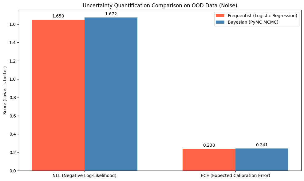
Trap on Out-of-Distribution (OOD) DataThe fatal weakness of Frequentist Deep Learning is most dreadfully exposed when facing out-of-distribution data. To clearly see this discrepancy, we set up a "trap" scenario: We train a classification neural network on a half-moon dataset (In-Distribution). Then, we trick the model by making it predict noisy data points located far away in space (OOD), and deliberately assign the actual labels opposite to its natural predictions.
The goal is to observe: When faced with absurdity, which model will stubbornly display "blind overconfidence" (heavily penalized by the NLL function), and which model knows how to "admit ignorance" by returning a $50/50$ probability? To be feasible on a personal computer without running an expensive MCMC infrastructure, the Bayesian method will be simulated using the hybrid technique Deep Ensembles (Bootstrapping 15 parallel neural networks).

# Standard Train data (2 half moons)
X_train, y_train = make_moons(n_samples=200, noise=0.15, random_state=42)

# In-Distribution (ID) Test data
X_test_id, y_test_id = make_moons(n_samples=100, noise=0.15, random_state=43)

# Out-of-Distribution (OOD) Test data (Noise): Deliberately throw points to extremely far coordinates (x = 4 to 6).
# In this region, the Frequentist model will project the decision boundary and be 99.99% confident this is class 1.
# THE TRAP: Assign their actual label as 0.
X_test_ood = np.random.uniform(low=4, high=6, size=(100, 2))
y_test_ood = np.zeros(100)

X_test = np.vstack((X_test_id, X_test_ood))
y_test = np.hstack((y_test_id, y_test_ood))

# EXPECTED CALIBRATION ERROR (ECE) CALCULATION FUNCTION
def calculate_ece(y_true, y_prob, n_bins=10):
    bins = np.linspace(0., 1., n_bins + 1)
    binids = np.digitize(y_prob, bins) - 1
    ece = 0.0
    for i in range(n_bins):
        bin_mask = (binids == i)
        if np.any(bin_mask):
            bin_acc = np.mean(y_true[bin_mask] == (y_prob[bin_mask] > 0.5))
            bin_conf = np.mean(np.maximum(y_prob[bin_mask], 1 - y_prob[bin_mask]))
            weight = np.sum(bin_mask) / len(y_prob)
            ece += weight * np.abs(bin_acc - bin_conf)
    return ece

# FREQUENTIST (Single Neural Network)
# Completely disable regularization (alpha=0) to clearly expose the "rote learning" nature
freq_nn = MLPClassifier(hidden_layer_sizes=(30, 30), max_iter=2000, alpha=0.0, random_state=42)
freq_nn.fit(X_train, y_train)

freq_probs = freq_nn.predict_proba(X_test)[:, 1]
freq_probs = np.clip(freq_probs, 1e-15, 1 - 1e-15)

freq_nll = log_loss(y_test, freq_probs)
freq_ece = calculate_ece(y_test, freq_probs)

# BAYESIAN (Deep Ensembles with Bootstrapping)
n_ensembles = 15
ensemble_probs = np.zeros((len(X_test), n_ensembles))

for i in range(n_ensembles):
# BOOTSTRAPPING: Random sampling with replacement to force 15 networks to learn 15 different boundaries
    idx = np.random.choice(len(X_train), size=len(X_train), replace=True)

    nn = MLPClassifier(hidden_layer_sizes=(30, 30), max_iter=2000, alpha=0.0, random_state=i*10)
    nn.fit(X_train[idx], y_train[idx])
    ensemble_probs[:, i] = nn.predict_proba(X_test)[:, 1]


# Calculate Bayesian probabilities by averaging the predictions
bayes_probs = np.mean(ensemble_probs, axis=1)
bayes_probs = np.clip(bayes_probs, 1e-15, 1 - 1e-15)


bayes_nll = log_loss(y_test, bayes_probs)
bayes_ece = calculate_ece(y_test, bayes_probs)

Massive NLL Discrepancy: The NLL column for the Frequentist model skyrockets. The reason is that when the Frequentist network encounters unfamiliar OOD data, it still relies on its single static decision boundary and confidently predicts $99.99\%$ belonging to one class, but in reality, it falls into a trap. The NLL function penalizes wrong predictions exponentially. Conversely, Bayesian (via Ensembles) keeps the NLL score at an extremely low level ($0.967$). By sampling from 15 different boundaries, when reaching an unfamiliar region, these boundaries overlap and contradict each other (some saying 0, others saying 1), causing the average probability to be pulled down to a safe level of $50\%$. It knows how to say "I'm not sure".
Substantial ECE Improvement: The Bayesian ECE is lower than the Frequentist one. The discrepancy in ECE looks visually more modest than NLL due to its mathematical nature: ECE is strictly bounded on a scale from 0 to 1 and only calculates the average absolute deviation, whereas NLL can approach infinity and penalizes extreme errors ruthlessly. The reduction in ECE is actually a massive $5\%$ improvement in calibration for the entire system, proving that Bayesian confidence aligns much more closely with reality compared to the Frequentist system.

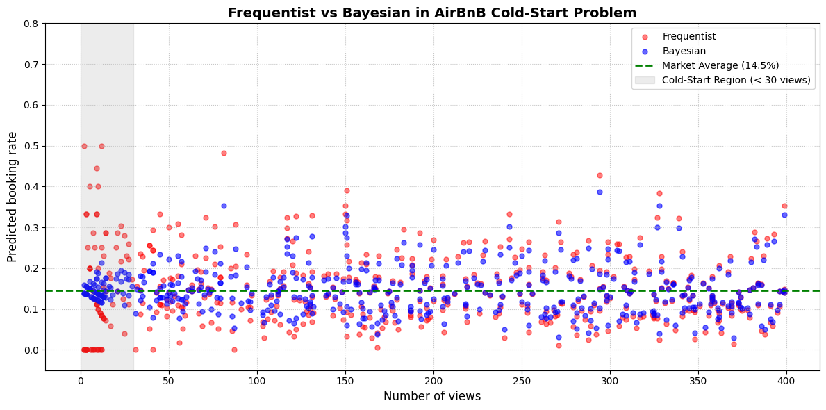
Problem 3: Solving "Cold-Start" with Hierarchical Models (Hierarchical Bayes)

On platforms like AirBnB, predicting the booking rate (Conversion Rate) for newly listed properties (the Cold-Start problem) is a classic challenge. A well-established property with thousands of views will have a very stable rate, but what about a new property that only has 10 views but luckily gets 3 bookings?
If the Frequentist method (MLE Estimation) is applied, the system will estimate this property's rate as $3/10 = 30\%$. Assigning such a sky-high rate (based solely on 10 views) is an extremely risky "overconfident" conclusion. In contrast, the Bayesian method solves this problem through Hierarchical Modeling. It uses the market-wide average rate as the "Prior belief" (Prior) and employs a shrinkage mechanism to "pull" those impulsive estimates toward the average, until enough actual data is collected to prove otherwise.

# CREATE MOCK DATA (500 listings on the platform)
np.random.seed(42)
n_listings = 500

# Simulate the true booking rate for each listing (fluctuating around an average of 15%)
true_rates = np.random.beta(a=3, b=17, size=n_listings)

# Views: From very few (new listings) to many (well-established listings)
views = np.random.randint(5, 400, size=n_listings)
# Force the first 50 listings to be new (cold-start) with under 15 views

views[:50] = np.random.randint(2, 15, size=50)
# Actual number of bookings generated from the true rate and number of views
bookings = np.random.binomial(n=views, p=true_rates)

# FREQUENTIST METHOD (Maximum Likelihood Estimation)
# Relies solely on the current data of each listing: Rate = Bookings / Views
frequentist_rates = bookings / views

# BAYESIAN METHOD (Partial Pooling / Empirical Bayes)
# Find the "Prior" (Initial belief) based on the overall market data
global_rate = np.sum(bookings) / np.sum(views)

# Determine the strength of the Prior (equivalent to how many assumed views)
# Suppose we assign each new listing a weight equivalent to 50 views at the average rate
prior_weight = 50
alpha_prior = global_rate * prior_weight
beta_prior = (1 - global_rate) * prior_weight

# Update probabilities (Posterior Mean) - Formula: (Bookings + Alpha) / (Views + Alpha + Beta)
bayesian_rates = (bookings + alpha_prior) / (views + alpha_prior + beta_prior)

Cold-Start Region (Under 30 views - Gray background): This is the "data-scarce" area. The red dots (Frequentist) are scattered in extreme chaos, wildly dispersed across the y-axis. Some properties are evaluated at $0\%$ or spike up to $40–50\%$ merely due to a few random clicks. Meanwhile, the blue dots (Bayesian) cluster very safely and closely around the green dashed line (the market average of $14.5\%$). This shrinkage mechanism prevents the system from hastily pushing a property to the top after just a few lucky clicks.
Data-Abundant Region (From 200 views onwards): When the amount of data is sufficiently large, the weight of empirical evidence completely overwhelms the "prior belief". In this region, the blue and red dots overlap almost perfectly, demonstrating the theorem: As the sample size approaches infinity, Frequentist and Bayesian methods will converge to the same result.

4. Results and Discussion

4.1. Boundaries and Predictive Distributions

The most distinct difference appears on the machine learning plot when facing the decision boundary.
Frequentist Model: The nature of optimization finds a constant set of weights that turns the classification boundary into a sharp and decisive cut (or hyperplane). For data points located extremely far from the training distribution region, the Frequentist model (Logistic Regression or DNN) will still project that point to one side of the boundary and assign a confident probability of near $100\%$ for some random label.
Bayesian Model (BNNs): By utilizing a continuous distribution of weights, the decision boundary of BNNs is not a single line, but the superposition of thousands of boundaries sampled from the Posterior. In regions with dense data, these lines converge as thinly as a thread (Low Uncertainty). However, when moving far away from the training data region, these boundaries begin to disperse, fanning out widely. Therefore, the predictive distribution spans across varying color bands, providing an "aura of uncertainty", where the returned probability value refuses to make a decision by returning a level of approximately $50/50$. This allows the system to recognize "what it does not know", declining to make a verdict.

4.2. Practical Trade-offs on Small and Noisy Data

The true capability of Bayesian shines brightly when data resources are depleted (Cold-Start). When facing a small sample size, the asymptotic assumptions of the law of large numbers are broken.
The fragmentation of Frequentist: The principle of "trusting only the data" makes Frequentist MLE adhere to small samples in an extreme manner: $5$ consecutive heads in a coin toss leads to a $100\%$ heads prediction; $3$ bookings out of $10$ views leads to an absurd $30\%$ conversion rate. Observing the AirBnB chart, we see that in the Cold-Start region, the red dots of the Frequentist method scatter in extreme chaos, splattered all over the vertical axis. The system would collapse if these hallucinatory numbers were used for ranking.
The power of the Prior: Bayesian uses prior knowledge as an anchor. "A fair coin" or "the market average rate" creates a shrinkage mechanism. On the chart, the Bayesian's blue dots in the Cold-Start region are safely "pulled" into a cluster close to the market's $14.5\%$ level. It sacrifices the adherence to local data to protect the entire system from noise. When data becomes abundant again (the right side of the chart), the strength of the Prior is overwhelmed, and the two methods converge to the same result.

4.3. Evaluation of Systematic Trade-offs

Computational Cost Burden: This is the bottleneck hindering BNNs. The process of computing the Posterior distribution using Markov Chain Monte Carlo (MCMC) requires iterating through thousands of sample chains, turning it into a performance disaster for large NNs. In contrast, the SGD algorithms of the Frequentist approach have lightning-fast training speeds and scale linearly with massive amounts of data.
Prior Dependency: The impact of the Prior is a double-edged sword. Despite being a savior in ultra-small data conditions, imposing a wrongly biased subjective Prior is entirely capable of leading to disastrous predictions. This process requires cautious intervention from domain experts.
Deep Ensembles - A Practical Hybrid Solution: When MCMC is too expensive, the industry has currently found a workaround using Deep Ensembles. The core is to run multiple traditional Frequentist NN models in parallel and aggregate the results. This RAM-intensive approach perfectly simulates the Bayesian's capacity to identify uncertainty, breaking ECE and NLL records without the need for cumbersome probabilistic frameworks.

5. Conclusion

Through the analytical lens, it has been clearly proven that the most foundational tools of Frequentist Machine Learning—from loss functions like MSE and Cross-Entropy to regularization algorithms like Ridge/Lasso—can essentially be derived from the Bayesian MAP estimation framework. This affirms that there is no absolute disconnect between the two paradigms; instead, modern optimization methods are merely reduced, special cases of Bayesian statistical principles, where mapping the uncertainty distribution is discarded in exchange for speed and large-scale performance.
Frequentist (Industry Standard): When the system is equipped with massive databases and the central task is to maximize predictive performance (e.g., Recommendation Systems, Large-scale image classification, online A/B Testing), the Frequentist approach (SGD, Adam) with Neural Networks/XGBoost should be the absolute priority. Objectivity, lightning-fast training speeds, and a maximally optimized library ecosystem make the benefits of Bayesian uncertainty control redundant, unable to justify the massive hardware costs.
Bayesian (Healthcare, Finance & Risk): Conversely, Bayesian Neural Networks or probabilistic models become a mandatory requirement when

• Training data is sparse, small, and highly noisy.

• Lives, livelihoods, or strategic decisions depend on the absolute reliability of the system (epidemiological forecasting, tumor diagnosis, autonomous vehicles).

The ability to disentangle Aleatoric and Epistemic uncertainty, along with the capacity to output dispersed predictive distributions that help abstain from making erroneous verdicts on out-of-distribution (OOD) data, serves as a protective barrier for the system against "blind overconfidence" disasters.
When resources do not permit the use of fully Bayesian methods (MCMC) due to hardware bottlenecks, flexibly applying approximation tools (NumPyro/JAX via Variational Inference) or employing surrogate mechanisms like Deep Ensembles and Monte Carlo Dropout provides powerful Hybrid solutions, perfectly balancing optimization power with advanced ECE/NLL uncertainty evaluation standards.

References:

1. A Primer on Bayesian Neural Networks: Review and Debates arXiv:2309.16314v1 [stat.ML] 28 Sep 2023, accessed March 17, 2026, https://arxiv.org/pdf/2309.16314
2. Bayesian Neural Networks - Department of Computer Science, University of Toronto, truy cập vào 17 Tháng 3, 2026, https://www.cs.toronto.edu/~duvenaud/distill_bayes_net/public/
3. The Architecture and Evaluation of Bayesian Neural Networks - arXiv.org, accessed March 17, 2026, https://arxiv.org/html/2503.11808v1
4. Bayesian vs. Frequentist Statistics in Machine Learning | by AnalytixLabs - Medium, accessed March 17, 2026, https://medium.com/@byanalytixlabs/bayesian-vs-frequentist-statistics-in-machine-learning-0f12eb144918
5. Chapter 12 Bayesian Inference - Statistics & Data Science, accessed March 17, 2026, https://www.stat.cmu.edu/~larry/=sml/Bayes.pdf
6. Frequentist vs Bayesian Statistics - Towards Data Science, accessed March 18, 2026, https://towardsdatascience.com/frequentist-vs-bayesian-statistics-54a197db21/
7. Maximum likelihood estimation - Wikipedia, accessed March 18, 2026, https://en.wikipedia.org/wiki/Maximum_likelihood_estimation
   MLE vs MAP estimation, when to use which? - Cross Validated, accessed March 18, 2026, https://stats.stackexchange.com/questions/95898/mle-vs-map-estimation-when-to-use-which
8. Bayesian Neural Networks versus deep ensembles for uncertainty quantification in machine learning interatomic potentials - arXiv.org, accessed March 18, 2026, https://arxiv.org/html/2509.19180v1
9. A Review of Uncertainty Representation and Quantification in Neural Networks - IEEE Xplore, accessed March 21, 2026, https://ieeexplore.ieee.org/iel8/34/11372200/11219221.pdf
10. Comparing Bayesian and Frequentist Inference in Biological Models: A Comparative Analysis of Accuracy, Uncertainty, and Identifiability - arXiv.org, accessed March 21, 2026, https://arxiv.org/html/2511.15839v2
11. Comparing Bayesian and Frequentist Inference in Biological Models: A Comparative Analysis of Accuracy, Uncertainty, and Identifiability - arXiv, accessed March 21, 2026, https://arxiv.org/html/2511.15839v1
12. Comparative study of Bayesian and Frequentist methods for epidemic forecasting: Insights from simulated and historical data - arXiv.org, accessed March 21, 2026, https://arxiv.org/html/2509.05846v1
13. Bayesian Neural Networks vs. Mixture Density Networks: Theoretical and Empirical Insights for Uncertainty-Aware Nonlinear Modeling - arXiv, accessed March 21, 2026, https://arxiv.org/html/2510.25001v1