
Linear Regression
In real work and daily life, we often ask the question:
"How can we predict an unknown value based on the data we already have?"
For example, if you have data about gold prices over the last 12 months, how can you estimate gold prices in the coming months?
This is where data analysis and machine learning become useful. Among them, linear regression is one of the simplest and most widely used methods.
1. What is Linear Regression?
Linear regression is a method used to predict a dependent variable (Y) based on an independent variable (X) through a linear function.
The model is represented by the equation:
$$y = f(x) = ax + b$$
Where:
a: slope, showing how much X affects Yb: interceptx: independent variabley: dependent variable
This equation describes the relationship between X and Y as a straight line on a coordinate plane.
In an ideal case, data points lie exactly on a straight line. In reality, data is noisy, influenced by many external factors, or scattered. Therefore, points rarely lie perfectly on a line; instead, they cluster around an average line.
When building a linear regression model, our goal is:
Find a line that best describes the trend of the data.
Specifically, that line should:
- Be close to most data points.
- Minimize the distance between actual values and predicted values.
- Produce the smallest overall error.
In other words, we look for the optimal line that represents the data.
With linear regression, we can forecast trends or analyze relationships between variables to support data-driven decisions. Common applications include predicting gold prices, stock prices, estimating revenue, analyzing academic performance, forecasting market demand, and more.
Linear regression is an important starting point in data analysis and machine learning. Although simple, it is highly effective for many real-world problems.
With the objective of minimizing prediction error, this process relies on two key tools: error measurement and optimization algorithms.
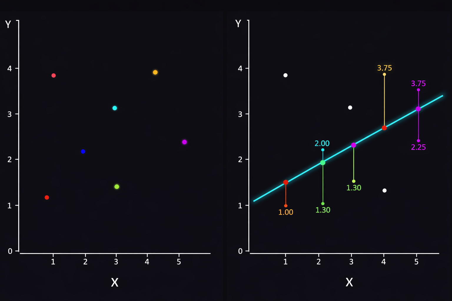
An example of the optimal line in linear regression.
1.1. Error Measurement - Loss Function
To know how "bad" our predicted line is, we need a concrete formula to measure error. The most common is MSE (Mean Squared Error).
- How it works: For each data point, compute the distance to the line and square it (to remove negatives and emphasize larger errors).
- Goal: The smaller the total squared error, the better the line fits the data.
1.2. Optimization Algorithm - Gradient Descent
After we have a way to measure error, how do we adjust the coefficients a and b so that the error decreases? This is where Gradient Descent comes in. Imagine standing on a mountain (high error) and trying to reach the valley (lowest error).
- Gradient (slope): tells the direction of steepest descent.
- Learning rate: the step size. Too large and you may overshoot; too small and learning is slow.
As a concrete example, this project focuses on predicting students' final exam scores based on a dataset about student performance.
2. Dataset Overview
2.1. Objective
The goal of this exercise is to build a linear regression model to predict the final score final_score based on study habits and previous exam scores. Since final_score is continuous, this is a classic regression problem.
We use the dataset student_performance_interactions.csv
Link: https://www.kaggle.com/datasets/spscientist/students-performance-in-exams
2.2. General Overview
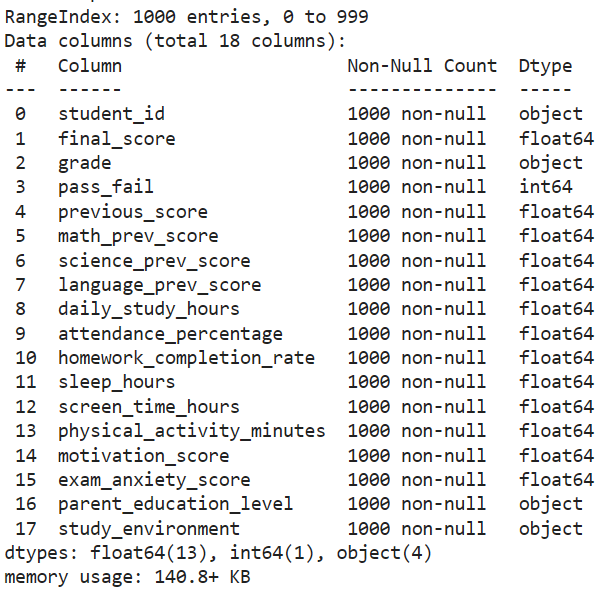
Overview of the dataset.
Size: 1000 student records with 18 columns
Quality: Complete data, no missing values, ready for further processing
Target variable: final_score (Actual score from 0 to 100)
2.3. Groups of Independent Variables
To achieve good performance, we group the features as follows:
Learning history (4 features):
previous_score: Overall previous average.math_prev_score: Previous Math score.science_prev_score: Previous Science score.language_prev_score: Previous Language score.
Study behavior (3 features):
daily_study_hours: Self-study hours per day.attendance_percentage: Attendance rate (%).homework_completion_rate: Homework completion rate (%).
Lifestyle & Health (3 features):
- sleep_hours: Sleep hours per night.
- screen_time_hours: Screen time hours.
- physical_activity_minutes: Physical activity minutes per day.
Psychology (2 features):
motivation_score: Study motivation score.exam_anxiety_score: Exam anxiety score.
Environment & Family (2 features - require encoding):
parent_education_level: Parent education level (categorical).study_environment: Study environment (categorical: Quiet, Moderate, Noisy).
2.4. Variables to Remove or Handle Separately
For this dataset, we remove the following variables to avoid misleading signals:
student_id: Identifier (no statistical meaning; remove during training).grade: Grade category (A, B, C...). This is derived fromfinal_score, so it should not be an input.pass_fail: Pass/Fail (0 or 1). Similar to grade, it is a consequence of the score, not a cause.
3. Simple Linear Regression (Single Variable)
First, after removing unnecessary variables, we check correlation and see that previous_score has the strongest impact on final_score.
target = 'final_score'
cols_to_check = list(df.columns[3:15])

corrs = {}
for col in cols_to_check:
    series = pd.to_numeric(df[col], errors='coerce')
    corr = df[target].corr(series)
    corrs[col] = corr

corr_df = pd.DataFrame.from_dict(corrs, orient='index', columns=['pearson_corr'])
corr_df = corr_df.sort_values('pearson_corr', key=lambda x: x.abs(), ascending=False)

print(corr_df)

correlation_results = corr_df
# Result
previous_score                 0.843755
math_prev_score                0.825755
science_prev_score             0.823998
language_prev_score            0.810688
attendance_percentage          0.737720
pass_fail                      0.484865
daily_study_hours              0.357275
homework_completion_rate       0.339800
motivation_score               0.255734
physical_activity_minutes     -0.044330
sleep_hours                    0.032623
screen_time_hours             -0.029856
3.1. Mathematical Explanation
The equation of a simple linear regression model is:
$$y = w_1x + w_0 + \epsilon$$
Where:
-
$y$: target value (label).
-
$x$: input feature.
-
$w_1$: slope (weight), indicating how much $x$ affects $y$.
-
$w_0$: intercept (bias), the value of $y$ when $x = 0$.
-
$\epsilon$: random noise.
For each data point $(x_i, y_i)$, the predicted value is:
$$\hat{y}_i = w_1x_i + w_0$$
The goal is to find $w_1$ and $w_0$ such that the distance between $\hat{y}$ (predicted) and $y$ (actual) is minimized.
We use MSE (Mean Squared Error) as the loss function. It is the average sum of squared errors between predictions and ground truth.
The loss function over $w_1, w_0$ should be minimized:
$$L(w) = \frac{1}{2n} \sum (y - \hat{y})^2 = \frac{1}{2n} \sum (y - w_1x - w_0)^2$$
Setting derivatives to zero:
Derivative w.r.t. $w_1$:
$$D_{w1} = \frac{-2}{n} \sum_{i=1}^{n} x_i(y_i - \hat{y}_i) = 0 \quad (1)$$
Derivative w.r.t. $w_0$:
$$D_{w0} = \frac{-2}{n} \sum_{i=1}^{n} (y_i - \hat{y}_i) = 0$$
$$\Leftrightarrow w_0 = \bar{y} - w_1\bar{x} \quad (2)$$
Substitute (2) into (1):
$$w_1 = \frac{\sum_{i=1}^{n} (x_i - \bar{x})(y_i - \bar{y})}{\sum_{i=1}^{n} (x_i - \bar{x})^2}$$
Then:
$$w_0 = \bar{y} - w_1\bar{x}$$
This method is called the Normal Equation. It finds the optimal $w_1, w_0$ in a single step without iteration. This solution acts as a benchmark to evaluate Gradient Descent in the next section.
3.2. Optimization Process (Gradient Descent)
Why choose Gradient Descent instead of the Normal Equation?
* Computational complexity: Normal Equation requires a matrix inversion with complexity $O(n^3)$. For large datasets or many features, this becomes slow and memory-heavy. Gradient Descent is much cheaper and scales better.
* Generality: Gradient Descent applies to many machine learning algorithms (e.g., neural networks) where no closed-form solution exists.
The update steps are:
Derivative w.r.t. $w_1$:
$D_{w1} = \frac{-2}{n} \sum_{i=1}^{n} x_i(y_i - \hat{y}_i)$
Derivative w.r.t. $w_0$:
$D_{w0} = \frac{-2}{n} \sum_{i=1}^{n} (y_i - \hat{y}_i)$
Update:
$$w_1 = w_1 - \alpha \times D_{w1}$$
$$w_0 = w_0 - \alpha \times D_{w0}$$
Repeat for many epochs until the error no longer decreases significantly.
4. Multiple Linear Regression
In practice, an outcome is influenced by many factors. Therefore, we extend the model from one variable $x$ to multiple features $x_1, x_2, ..., x_n$.
General equation:
$$y = w_0 + w_1x_1 + w_2x_2 + ... + w_nx_n + \epsilon$$
4.1. Data Preparation
Based on the source analysis from linear_regression1.ipynb, the data preparation process is:
- Target (y):
final_score - Features (X): 12 numerical features.
- Unnecessary or unencoded columns (
student_id,grade,pass_fail,parent_education_level,study_environment) are removed. - The 12 features used are:
previous_score,math_prev_score,science_prev_score,language_prev_score,daily_study_hours,attendance_percentage,homework_completion_rate,sleep_hours,screen_time_hours,physical_activity_minutes,motivation_score,exam_anxiety_score.
- Unnecessary or unencoded columns (
4.2. Implementing Gradient Descent
Before using a library, we implement linear_regression_gd to understand how Gradient Descent works with multiple features.
- Initialization: weights $w$ are initialized to 0.
- Loop (epochs):
- Predict: $\hat{y} = Xb \cdot w$
- Error: $error = \hat{y} - y$
- Gradient: $\nabla w = \frac{2}{n} Xb^T \cdot error$
- Update: $w = w - \alpha \cdot \nabla w$
- Early stopping if the loss change is negligible.
def linear_regression_gd(X, y, lr=0.05, epochs=2000, tol=1e-6):
    Xb = add_bias(X)
    n, d = Xb.shape
    w = np.zeros(d)
    loss_history = []
    prev_loss = float('inf')
    start = time.time()
    for epoch in range(epochs):
        y_pred = Xb @ w
        error = y_pred - y
        grad = (2/n) * (Xb.T @ error)
        w -= lr * grad
        loss = mse(y, y_pred)
        loss_history.append(loss)
        if abs(prev_loss - loss) < tol:
            break
        prev_loss = loss
    train_time = time.time() - start
    return w, loss_history, epoch+1, train_time
4.3. Implementation with Scikit-Learn
Instead of manually computing derivatives for multiple variables, we use the highly optimized scikit-learn library.
from sklearn.linear_model import LinearRegression
from sklearn.metrics import mean_squared_error, mean_absolute_error, r2_score
from sklearn.preprocessing import StandardScaler

# Reuse the same split as GD
Xtr = X_train
Xte = X_test
ytr = y_train
yte = y_test

# Scale using train stats only
scaler = StandardScaler()
Xtr_std = scaler.fit_transform(Xtr)
Xte_std = scaler.transform(Xte)

# Train
start = time.time()
model = LinearRegression()
model.fit(Xtr_std, ytr)
sk_time = time.time() - start

# Predict
yte_pred = model.predict(Xte_std)
5. Code
Below is the GitHub link with the full code for this linear regression project (simple regression, multiple regression, and scikit-learn implementation):
https://github.com/atognoob/AIO2026/tree/main/3_Project1
Chưa có bình luận nào. Hãy là người đầu tiên!