1. Introduction
Anyone working with Machine Learning has likely encountered a seemingly absurd paradox: a high-end, sophisticated model yields poor results, while an average model performs surprisingly well. It sounds hard to believe, but the truth is: the cause does not lie in the algorithm, but in how we handle the input data.
In other words, the model isn't wrong—the data is what determines what it learns.
Andrew Ng, a world-renowned AI expert, once stated:
"Coming up with features is difficult, time-consuming, requires expert knowledge. 'Applied machine learning' is basically feature engineering."

This statement highlights a crucial truth: algorithms are merely tools, while data quality and how we "tell the story" to the model are the core factors. If the input data does not accurately reflect the nature of the problem, then no matter how optimized the algorithm is, it will only learn biased or superficial relationships.
This article will explain why Feature Engineering is incredibly important in Machine Learning problems, accompanied by visual illustrations.
2. What is Feature Engineering?
Feature Engineering is the process of designing and selecting features that accurately reflect the nature of the problem, helping Machine Learning models operate more effectively.
This process typically includes the following key groups of tasks:
- Feature Transformation: Transforming existing features (e.g., using Logarithms to handle skewed data, or Scaling to bring data into the same value range).
- Feature Creation: Creating new features from old data (e.g., calculating "Distance" from "Longitude" and "Latitude").
- Feature Selection: Removing features that cause noise or do not contribute value, making the model more compact.
- Feature Extraction: Reducing data dimensionality (such as PCA) to extract the most core information from a complex dataset.
3. Why is Feature Engineering extremely important?
- Improving model performance
The quality of input features has a direct influence on the performance of the machine learning model. Good feature engineering helps the model detect meaningful patterns in the data, thereby improving both accuracy and generalization ability on the data.
A typical example is the house price prediction problem. If directly using the construction year variable (1995, 2000, 2002), the model must self-infer the relationship between this number and the house value - a non-linear relationship and dependent on the current time. Meanwhile, converting this variable into house age (current year minus construction year) helps the feature become more intuitive and meaningful, reflecting directly the depreciation level and usage value of the house. Thanks to that, the model is easier to learn, converges faster, and usually gives more accurate prediction results.
- Increasing the suitability of data with algorithms
In reality, many models only work effectively when input data is represented under a suitable numerical format and has a stable distribution. If the house number is in tens while the price is in billions, distance-based algorithms will be overwhelmed by the price feature and ignore the remaining feature.
Feature engineering plays the role of a bridge between real-world data and the mathematical requirements of the algorithm, putting features onto a "level playing field". Through Feature transformation techniques, data is more compatible with the algorithmic model, helping increase learning efficiency.
- Reducing complexity and training time
Raw data can contain redundant features, causing noise and making the model spend training time on non-useful information. This not only increases training time but can also cause the overfitting problem (rote learning noisy data).
Through Feature engineering, data is standardized and the input space is dimensionally reduced effectively, helping the model only focus on features containing much information. Thanks to that, computational resources (RAM/CPU) and training time are optimized.
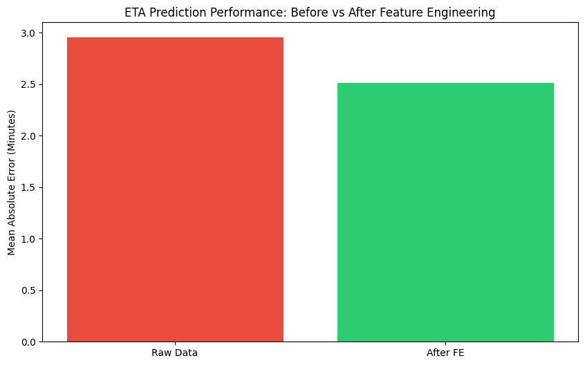
4. Performance Evaluation: With and without Feature Engineering
The following brief example demonstrates the difference in performance when Feature Engineering is applied versus when it is not in a Machine Learning (ML) task.
Context: In the tech-transport sector, accurately predicting the Estimated Time of Arrival (ETA) is a critical factor for reducing cancellation rates and optimizing the customer experience. We will simulate an ETA prediction problem.
-
The difference between raw data and processed data
- Raw Data: Utilizes only the original
variables:Distance_km(Distance),Hour(Time of day),
andIs_Raining(Rain status). While the model has access
toHourandIs_Raining, it must attempt to uncover the complex
relationships between them entirely on its own. It tends to treat
rush hour similarly to any other time frame, lacking the ability to
"emphasize" these sensitive periods. - After Feature Engineering: We incorporate additional features derived from Domain Knowledge.
Is_Rush_Hour(Rush Hour): Groups specific time frames (7–9 AM and 4–7 PM) to explicitly identify them as peak traffic congestion periods.Rain_Impact(Impact of Rain): This is an Interaction Feature. It helps the model understand that: Rain at night does not affect travel time as severely as rain during rush hour.
- Raw Data: Utilizes only the original
-
Python demo code: Performance comparison
This code snippet simulates the training of two models: one utilizing only the initial raw data and another utilizing the processed features.
import pandas as pd
import numpy as np
import matplotlib.pyplot as plt
from sklearn.ensemble import RandomForestRegressor
from sklearn.metrics import mean_absolute_error

# 1. Simulate Uber/Grab-like data
data = {
    'Distance_km': [2, 5, 2, 8, 3, 10, 2, 6, 1, 4, 3, 7],
    'Hour': [8, 8, 23, 17, 12, 18, 2, 17, 9, 21, 8, 16],
    'Is_Raining': [1, 0, 0, 1, 0, 1, 0, 0, 1, 0, 1, 0],
    'Actual_ETA': [18, 20, 6,  45, 10, 55, 5,  25, 12, 12, 22, 28] # Actual travel time (minutes)
}
df = pd.DataFrame(data)

# --- BEFORE FEATURE ENGINEERING ---
X_raw = df[['Distance_km', 'Hour', 'Is_Raining']]
model_raw = RandomForestRegressor(n_estimators=100, max_depth=3, random_state=42).fit(X_raw, df['Actual_ETA'])
mae_raw = mean_absolute_error(df['Actual_ETA'], model_raw.predict(X_raw))

# --- AFTER FEATURE ENGINEERING ---
# Create feature 'Is_Rush_Hour': peak hours from 7–9 AM and 4–7 PM
df['Is_Rush_Hour'] = df['Hour'].apply(lambda x: 1 if (7 <= x <= 9) or (16 <= x <= 19) else 0)
# Create feature 'Rain_Impact': combined effect of rain during rush hour
df['Rain_Impact'] = df['Is_Raining'] * df['Is_Rush_Hour']

X_fe = df[['Distance_km', 'Hour', 'Is_Raining', 'Is_Rush_Hour', 'Rain_Impact']]
model_fe = RandomForestRegressor(n_estimators=100, max_depth=3, random_state=42).fit(X_fe, df['Actual_ETA'])
mae_fe = mean_absolute_error(df['Actual_ETA'], model_fe.predict(X_fe))

# 2. Plot error comparison (Visualization)
labels = ['Raw Data', 'After FE']
errors = [mae_raw, mae_fe]

plt.figure(figsize=(10, 6))
bars = plt.bar(labels, errors, color=['#e74c3c', '#2ecc71'])
plt.ylabel('Mean Absolute Error (Minutes)')
plt.title('ETA Prediction Performance: Before vs After Feature Engineering')
plt.show()
- Evaluation Chart
When running the code above, you will see the Mean Absolute Error (MAE) decrease significantly:
5. Core techniques in Feature Engineering
Data Preprocessing
Before talking about feature engineering, we need to do something far less glamorous: clean the data.
Overall objective
In practice, data is rarely tidy from the start. Missing values, inconsistent formats, and even duplicated records are the norm rather than the exception. Preprocessing is the step that makes data safe to work with before we attempt to make it useful for machine learning models.
If preprocessing is skipped, several issues may occur:
-
The model may fail to train
-
Statistical measures can be distorted
-
The model may learn noise instead of signal
For this reason, preprocessing is not about “making the data look nice”, but about ensuring that the data faithfully represents the problem and can be learned from in a stable way.
1. Handling missing values
Purpose
Most machine learning algorithms assume that every input is a valid value. Even a single null value can cause training to fail. Even when an algorithm technically supports missing values, they often distort basic statistics such as means, variances, and correlations. Therefore, we must ensure that the dataset does not contain missing values that break training or bias analysis.
Missing values typically arise due to:
-
Users not providing information
-
Data collection errors
-
Fields that are not applicable to all entities
Common techniques
- Imputation
- Median imputation: Used for numerical variables. The median is less sensitive to extreme values than the mean, making it safer for skewed distributions or data with outliers.
- Mode imputation: Used for categorical variables. Missing values are replaced with the most frequent category, preserving valid labels without introducing artificial values.
df['age'] = df['age'].fillna(df['age'].median())

df['city'] = df['city'].fillna(
    df['city'].mode()[0]
)
- Dropping features: When a column contains too many missing values and carries little information, removing it entirely may be more reasonable than imputing.
2. Handling outliers: Remove or Preserve?
Purpose
Outliers matter because they can strongly influence statistics and model behavior. Some algorithms are highly sensitive to extreme values, while others may overfit to rare but unimportant cases. However, not all outliers are errors. Many extreme values reflect genuine, rare real-world events.
A simple way to inspect outliers is to visualize the data distribution. Below is an example using Titanic ticket fares:
sns.boxplot(titanic['fare'].dropna())
plt.title("Fare distribution")
plt.show()
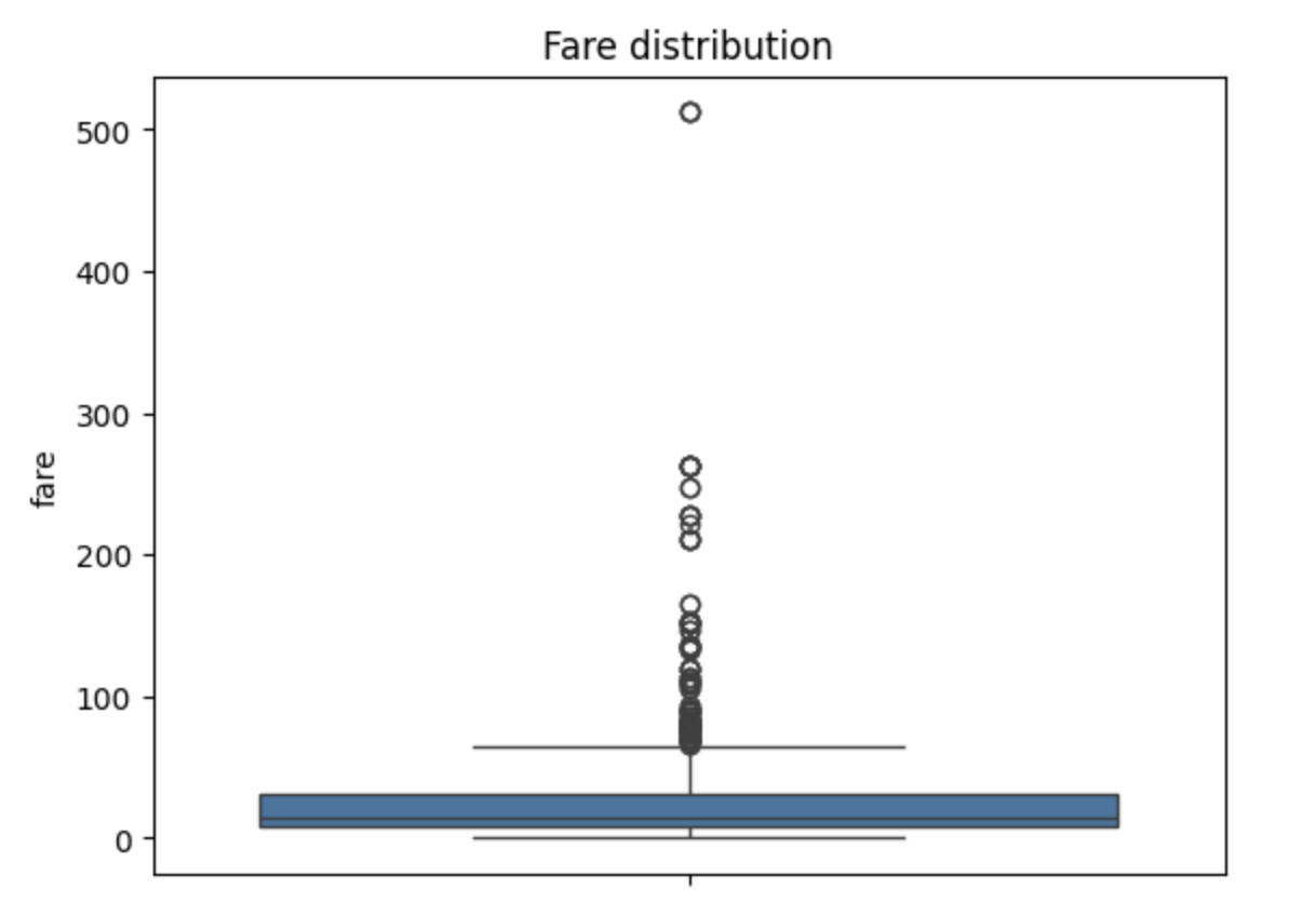
The plot shows several extremely high fares. At first glance, these look like classic outliers. However, deciding whether they are noise or signal requires domain context.
On the Titanic, ticket prices varied drastically between classes. First-class passengers paid significantly more than others, and those high values reflect real socioeconomic differences rather than data errors.
In this case, removing high fares would erase meaningful information about passenger class and wealth, factors that are likely correlated with survival. For that reason, we choose not to remove outliers at the preprocessing stage. This illustrates an important principle of preprocessing:
Preprocessing is about protecting the integrity of the data, not forcing it to look “nice.”
Common techniques
When outliers need to be handled, we can:
- Remove outliers entirely: Appropriate when extreme values are clearly invalid and represent noise rather than meaningful variation. A common method is the Interquartile Range approach. (GeeksforGeeks, 2025).
q1 = titanic['fare'].quantile(0.25)
q3 = titanic['fare'].quantile(0.75)
iqr = q3 - q1

df_no_outliers = titanic[
    (titanic['fare'] >= q1 - 1.5 * iqr) &
    (titanic['fare'] <= q3 + 1.5 * iqr)
]
- Replacing or capping extreme values: Limit how extreme values are allowed to be. This preserves sample size while reducing the influence of rare extremes.
# Capping extreme values
df['fare_capped'] = df['fare'].clip(
    lower=q1 - 1.5 * iqr,
    upper=q3 + 1.5 * iqr
)

# Transforming distribution
titanic['fare_log'] = np.log1p(titanic['fare'])
3. Formatting and Type consistency
Purpose
Ensure that the data has consistent formatting to avoid misinterpretation during analysis and training. A quick way to inspect column types is using dtypes.
Common issues include:
-
Datetime stored as strings
-
Inconsistent categorical labels (
"Male"vs"male") -
Numbers stored as text
Standardizing data types
- Datetime normalization
df['purchase_date'] = pd.to_datetime(df['purchase_date'])
- String normalization
df['gender'] = df['gender'].str.lower().str.strip()
4. Deduplication
Purpose
Duplicate data does not break code, but it biases models by over-representing certain observations. This makes deduplication a simple but valuable safety check.
Duplicates often arise from:
-
Multiple logging events
-
Merging data from multiple sources
-
Errors in data pipelines
If left untreated, duplicates can:
-
Inflate certain observations
-
Distort data distributions
-
Mislead the model about real frequencies
Duplicates don’t break code, but they do bias models by over-representing certain samples. Because of that, deduplication is a quick but important safety check.
# Check duplicated rows
df.duplicated().sum()

# Remove duplicates
df = df.drop_duplicates()
5.1. Feature transformation: Making data model-friendly
Overall objective
After preprocessing, the data is clean and reliable. But clean does not mean learnable.
Machine learning models do not understand meaning or context—they understand numbers and geometry. Feature transformation is the step where we restructure clean data so that mathematical models can actually learn from it.
The goal is to make features:
-
Comparable in scale
-
Numerically meaningful
-
Easier to optimize
-
Less sensitive to skewed distributions
1. Scaling numerical features
Purpose
In many problems, numerical features have very different units and ranges. Models such as logistic regression, SVMs, and neural networks are particularly sensitive to feature magnitude.
Example:
| Feature | Value range |
|---|---|
| Age | 0 – 80 |
| Income | 1,000 – 200,000 |
| Distance | 0 – 10 |
However, we should not scale:
-
Binary variables (0 / 1)
-
Ordinal variables unless explicitly encoded
Common techniques
- Standardization (Z-score scaling)
Standardization rescales data to have mean 0 and standard deviation 1.
$$
z= \frac{x - \mu}{\sigma}
$$
Where:
-
$z$ : original feature value
-
$\mu$ : feature mean
-
$\sigma$ : standard deviation
from sklearn.preprocessingimport StandardScaler

scaler = StandardScaler()
df['price_scaled'] = scaler.fit_transform(df[['price']])
This method is particularly suitable for linear models, SVMs, neural networks, and gradient-based optimization algorithms.
- Normalization (Min-Max scaling)
Min–Max scaling rescales values into the range $[0, 1]$
$$
x′= \frac{x - x_{\min}}{x_{\max} - x_{\min}}
$$
Characteristics:
-
Preserves distribution shape
-
Easy to interpret
-
Suitable when feature bounds are known
However, it is highly sensitive to outliers.
from sklearn.preprocessingimport MinMaxScaler

scaler = MinMaxScaler()
df['price_minmax'] = scaler.fit_transform(df[['price']])
- Robust scaling
When data contains many outliers, RobustScaler is safer. It uses the median and IQR instead of mean and standard deviation.
from sklearn.preprocessingimport RobustScaler

scaler = RobustScaler()
df['price'] = scaler.fit_transform(df[['price']])
2. Encoding categorical features
Purpose
Machine learning models cannot work directly with strings such as "male" or "female". Categorical features must be converted into numerical form without introducing artificial ordering.
Common techniques
- One-hot encoding
Safest option for nominal categories. It creates binary columns without imposing order.
pd.get_dummies(df, columns=['color'], drop_first=True)
- Label encoding
Assigns numbers to categories. This is only appropriate for ordinal data. Applying label encoding to unordered categories introduces serious bias.
education_map = {
    'High school': 0,
    'Bachelor': 1,
    'Master': 2,
    'PhD': 3
}

df['education_encoded'] = df['education'].map(education_map)
3. Transforming skewed distributions
Purpose
Many real-world features are right-skewed, with many small values and a few extremely large ones. Such distributions can:
-
Slow model convergence
-
Hurt linear model performance
-
Overemphasize rare cases
Instead of removing outliers, we reshape the distribution using transformations such as logarithms.
import numpy as np

df['fare_log'] = np.log1p(df['fare'])
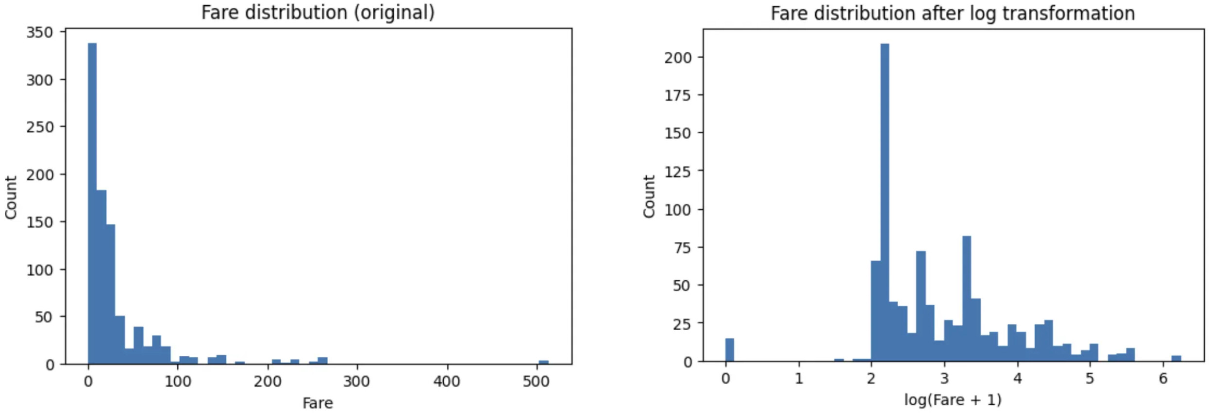
To demonstrate, we can see that the extreme values dominate the scale and compress the majority of the data into a narrow range in the original one. After the log:
-
Extreme values are compressed rather than removed
-
The bulk of the data is more evenly spread
-
The distribution becomes closer to symmetric
-
The relative ordering of values is preserved.
4. Discretization
Purpose
Discretization means converting a continuous numerical feature into a small number of categories (bins). This is useful when:
-
Exact values are noisy.
For example, in working age group, treating age as an exact number may introduce unnecessary noise into the model, as a 29-year-old is not really different from a 30-year-old. -
The relationship with the target is not linear.
-
Human-defined ranges carry meaning
Some ranges naturally mean something. In age group, we have children, teenagers, adults, and seniors. These groups are socially and behaviorally distinct. So discretization lets us inject this real-world knowledge directly into the data.
Example: age groups (child, adult, senior)
df['age_group'] = pd.cut(
    df['age'],
    bins=[0, 12, 18, 35, 60, 100],
    labels=['child', 'teen', 'adult', 'middle_aged', 'senior']
)
At this point, age stops being a precise measurement and becomes a conceptual category.
On the other hand, we should avoid discretization when:
-
Using tree-based models (they handle non-linearity well)
-
The exact numeric value is meaningful
-
We already have enough data for smooth learning
That said, discretization is not a default step. It’s a tool, not a requirement.
5.2. Feature Creation & Extraction
Overall Objective
The core goal of this section is to transform raw data into more meaningful information for machine learning models. On the same dataset, different feature engineering strategies can lead to completely different model outcomes, even when the learning algorithm remains unchanged. This is why Feature Engineering often plays a more critical role than model selection itself.
In this section, we clearly distinguish between two concepts:
-
Feature Creation: Manually creating new features using domain knowledge and business logic.
-
Feature Extraction: Automatically transforming complex data (e.g., text, images) into numerical vector representations using algorithms.
1. Feature Creation: Creating Features from Domain Knowledge
Feature Creation is the process of combining, transforming, or inferring new features from existing ones to better reflect the underlying problem.
Key characteristics:
-
Not generated automatically by algorithms
-
Actively designed by humans
-
Strongly dependent on domain knowledge
Commonly used operations include:
| Type | Example |
|---|---|
| Sum | A + B |
| Difference | A - B |
| Ratio | A / B |
| Interaction | A * B |
| Log / Power | log(A), A², √A |
import pandas as pd

df = pd.DataFrame({
    "weight_kg": [60, 72, 80],
    "height_m": [1.65, 1.70, 1.75],
    "A": [10, 20, 30],
    "B": [2, 5, 6],
})

df["BMI"] = df["weight_kg"] / (df["height_m"] ** 2)
df["A_plus_B"] = df["A"] + df["B"]
df["A_div_B"] = df["A"] / df["B"]
df["A_mul_B"] = df["A"] * df["B"]
Real-world examples:
These features usually do not exist in raw data but directly capture the essence of the business problem.
-
Sales problems
-
Revenue = Price × Quantity -
Discount rate = Discount / Original price -
Revenue per customer
-
-
Healthcare problems (BMI example)
Weight and height alone are weak indicators, but BMI provides a much more accurate measure of body condition:
$$
\mathrm{BMI}=\frac{\text{Weight (kg)}}{\text{Height (m)}^2}
$$
-
If only
weightandheightare provided, the model may learn this relationship, but it requires more data and is more prone to overfitting. -
Providing BMI explicitly reduces model complexity, improves interpretability, and increases learning efficiency.
Feature Creation in Practice
| Domain | Example Features |
|---|---|
| Finance | Debt / Income, Volatility |
| Marketing | CTR, Conversion Rate |
| Education | GPA, Completion rate |
| E-commerce | Discounted price, Price per item |
| Computer Vision | Aspect ratio, Object density |
| NLP | Sentence length, Keyword count |
2. Feature Extraction: Extracting Features from Complex Data
Feature Extraction uses algorithms to transform unstructured or high-dimensional data into numerical vectors that models can learn from.
Key characteristics:
-
Algorithm-driven
-
Applied to: Datetime, Text, Image, Audio, High-dimensional numerical data
a. Feature Extraction from Datetime
Datetime data should not be left as raw timestamps. Instead, it can be decomposed into multiple informative features that are extremely powerful for demand forecasting and behavioral analysis.
Example timestamp: 2025-01-21 19:30:00
Extractable features include:
| Feature | Meaning |
|---|---|
| Day of week | Weekly patterns |
| Is weekend | Different weekday/weekend behavior |
| Month | Seasonality |
| Quarter | Business cycles |
| Hour | Time-of-day behavior |
| Season | Spring / Summer / Fall / Winter |
import pandas as pd

df = pd.DataFrame({
    "timestamp": pd.to_datetime([
        "2025-01-21 19:30:00",
        "2025-03-02 08:10:00"
    ])
})

df["dow"] = df["timestamp"].dt.dayofweek        # 0=Mon ... 6=Sun
df["month"] = df["timestamp"].dt.month
df["quarter"] = df["timestamp"].dt.quarter
df["is_weekend"] = (df["dow"] >= 5).astype(int)
b. Feature Extraction from Text
Text is unstructured data and must be converted into numerical vectors. Two classical methods are Bag of Words (BoW) and TF-IDF.
| Criterion | Bag of Words (BoW) | TF-IDF |
|---|---|---|
| Core idea | Count word occurrences | Balance word frequency with global rarity |
| Representation | Count vector | TF × IDF weighted vector |
| Sparsity | Very sparse | Very sparse |
| Effect of stopwords | Strongly affected | Down-weighted |
| Advantages | Simple, intuitive, easy to implement | More powerful than BoW |
| Limitations | Cannot distinguish important words | Still linear, no context |
| Complexity | Low | Low–Medium |
| Best for | Baselines, simple tasks | Text classification, search, clustering |
| Common libraries | CountVectorizer | TfidfVectorizer |
c. Feature Extraction from Images
Images are high-dimensional data (H × W × C). Common approaches include:
-
Flattening pixels: Old approach, inefficient
-
Color histograms: Capture color distribution
-
CNN / Vision Transformers (modern):
- Output: Embedding vectors (e.g., 512, 768, 1024 dimensions)
- Use cases: Classification, retrieval, clustering, similarity search
- These embeddings preserve semantic information of images
d. PCA (Principal Component Analysis)
PCA is a dimensionality reduction technique.
-
Mechanism: Creates new orthogonal axes (principal components) that
capture the maximum variance. -
Goal: Retain only the most informative components.
-
Intuition: PCA rotates the coordinate system so the data can be represented most clearly with fewer dimensions.
Summary: Feature Creation vs Feature Extraction
| Feature Creation | Feature Extraction |
|---|---|
| Human-driven | Algorithm-driven |
| Domain/business-oriented | Mathematical |
| Highly interpretable | Less interpretable (black-box) |
| Usually low-dimensional | Can be very high-dimensional |
| Crucial for tabular & business data | Essential for AI (text, image, audio) |
5.3. Feature Selection
Overall Objective
The goal of Feature Selection is to retain features that truly help prediction and remove those that introduce noise.
Unlike previous steps:
-
It does not create new features (as in Feature Creation).
-
It does not transform existing data (as in Feature Extraction).
-
It focuses on the core question: “Which features are actually necessary for the model?”
After creating new features and extracting features from complex data, a common issue arises: the number of features grows too large. Not all features improve model performance. On the contrary, redundant or irrelevant features often slow down training and increase the risk of overfitting. Feature Selection helps the model “carry less weight” by filtering out noise.
Note:
In practice, there are many feature selection techniques (Filter, Wrapper, Embedded). However, the most fundamental and widely used approach is Filter Methods, which rely on statistical properties to eliminate useless features before model training.
Below are four types of features that should be removed.
1. Removing Low-Variance Features
These are features whose values are almost constant across the dataset. If a feature does not vary, the model cannot learn anything meaningful from it.
Example: In an HR dataset with 1,000 employees:
-
Column
Nationality: 999 are"Vietnam", only 1 is"Other" -
Column
Is_Human: 100% are"Yes"
Such features contain nearly zero information and should be removed first.
2. Removing Irrelevant Identifier Features (IDs)
These features carry no predictive information about the target variable.
Example: A house price prediction dataset with the following columns:
| Feature | Description |
|---|---|
| Area | Floor area |
| Rooms | Number of rooms |
| Distance | Distance to city center |
| House_ID | House identifier |
Python code:
import numpyas np
import pandasas pd

np.random.seed(42)
n =200

# House_ID is only an identifier (no predictive meaning)
df_house = pd.DataFrame({
"House_ID": np.arange(1, n +1),
"Area": np.random.normal(80,20, n).clip(30,200),
"Rooms": np.random.randint(1,6, n),
"Distance": np.random.normal(8,3, n).clip(0.5,25),
})

# Price depends on Area, Rooms, Distance + noise
noise = np.random.normal(0,15, n)
df_house["Price"] = (
2.5 * df_house["Area"]
    +18 * df_house["Rooms"]
    -6 * df_house["Distance"]
    + noise
)

# Remove ID column by rule
drop_cols = ["House_ID"]
X = df_house.drop(columns=drop_cols)
In this problem, Area, Rooms, and Distance are directly related to house price. In contrast, House_ID is merely an identifier. Even though each value is unique, it contains no information about price and should be removed immediately to avoid confusing the model.
3. Removing Features with Low Correlation to the Target
Features with very low correlation to the target variable usually act as noise rather than signal.
Example: In a sales revenue prediction problem:
| Feature | Correlation with Revenue |
|---|---|
| Marketing_Spend | 0.62 |
| Store_Size | 0.48 |
| Employee_ID | 0.01 |
Python code
corr = df.corr(numeric_only=True)["Revenue"].drop("Revenue")
print(corr)
Output:
Marketing_Spend    0.62
Store_Size         0.48
Employee_ID        0.01
Employee_ID has a correlation close to zero with revenue, indicating that it provides almost no predictive information. Keeping this feature would only add noise, so it should be removed.
4. Removing Multicollinear Features
Multicollinearity occurs when input features have strong linear dependencies among themselves. This causes instability in models - especially linear regression, because the same information is duplicated across multiple features.
Example: In a customer behavior analysis dataset:
| Feature | Meaning |
|---|---|
| Total_Purchases | Total number of purchases |
| Total_Spending | Total amount spent |
| Avg_Order_Value | Average value per order |
Python code:
import pandasas pd

df = pd.DataFrame({
"Total_Purchases": [5,10,15,20],
"Avg_Order_Value": [20,22,21,23],
})

df["Total_Spending"] = df["Total_Purchases"] * df["Avg_Order_Value"]
df.corr()
Mathematically, there is a clear relationship:
$$
\text{Total\_Spending} \approx \text{Total\_Purchases} \times \text{Avg\_Order\_Value}
$$
If all three features are included, model coefficients become unstable due to redundant information. A reasonable selection strategy would be:
-
Keep
Total_Spending(it directly reflects customer value—the ultimate target). -
Remove
Total_PurchasesorAvg_Order_Value(or both), depending on which feature is more relevant to the target.
6. Conclusion
Modern Machine Learning algorithms are becoming increasingly powerful and more accessible than ever. With just a few lines of code, we can now apply advanced models such as XGBoost, Random Forests, or even Deep Learning. However, algorithms cannot understand data if the input does not carry the right information. A model can only learn from what we feed into it, and that is the core role of Feature Engineering.
Feature Engineering transforms raw data into data that is learnable. From creating features that reflect the true nature of the problem, to extracting meaningful representations from complex data, and finally to removing redundant or noisy features, every step directly impacts model quality. In many real-world scenarios, a simple model with well-designed features can outperform a complex model built on poor features.
More importantly, Feature Engineering is not a purely technical step. It is a combination of data understanding, domain knowledge, and modeling intuition. This is also where the experience of a data practitioner becomes most visible, as there is no universal formula that works for every problem.
Therefore, when asking the question “Is Feature Engineering more important than the algorithm?”, the answer for most practical Machine Learning problems is: yes. Strong algorithms are necessary, but strong features are the foundation. Once the data is properly designed, choosing an algorithm often becomes an optimization step rather than the determining factor of success or failure.
7. References
-
GeeksforGeeks. (2025). Interquartile Range to detect outliers in data.
https://www.geeksforgeeks.org/machine-learning/interquartile-range-to-detect-outliers-in-data. (GeeksforGeeks) -
Theng, D., & Bhoyar, K. K. (2023). Feature selection techniques for machine learning: a survey of more than two decades of research. Knowledge and Information Systems.
https://link.springer.com/article/10.1007/s10115-023-02010-5(Springer) -
Poslavskaya, E., & Korolev, A. (2023). Encoding categorical data: Is there yet anything ‘hotter’ than one-hot encoding? arXiv.
https://arxiv.org/abs/2312.16930(arXiv) -
Guo, C., & Berkhahn, F. (2016). Entity Embeddings of Categorical Variables. arXiv.
https://arxiv.org/abs/1604.06737(arXiv)
Chưa có bình luận nào. Hãy là người đầu tiên!