Anomaly Detection in Time Series Data

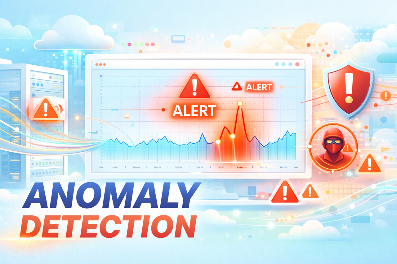Figure 1. Anomaly Detection in life (the figure is generated by ChatGPT).

This survey is summarized and rewritten based on the below publication.

[1] Boniol, P., Liu, Q., Huang, M., Palpanas, T., & Paparrizos, J. (2024). Dive into time-series anomaly detection: A decade review. arXiv. https://arxiv.org/abs/2412.20512]

Recent advances in data acquisition technologies, together with the ever-increasing volume and velocity of streaming data, have underscored the essential need for time series analysis methods. In this context, anomaly detection in time series data has become an important research direction, with numerous applications in domains such as cybersecurity, financial markets, law enforcement, and healthcare.

Figure 2. The applications of time-series data in life (the figure is generated by Artlist.io).

Whereas traditional research on anomaly detection has primarily relied on statistical measures, the rapid growth of machine learning algorithms in recent years has created the need for a systematic and general framework to characterize research methods for time series anomaly detection. This survey groups and summarizes existing anomaly detection approaches based on a process-centric taxonomy in the time series context.

In addition to proposing a systematic taxonomy of anomaly detection methods, this study conducts a meta-analysis of related work and highlights common trends in time series anomaly detection.

Concepts and Taxonomy of Anomalies

Definition of Anomalies

The rapid growth in both the number and practical deployment of sensors, networks, and cost-efficient data storage and processing systems has driven the need to collect and store massive volumes of time-dependent data. Recording such data gives rise to an ordered sequence of real-valued observations, commonly referred to as a time series.

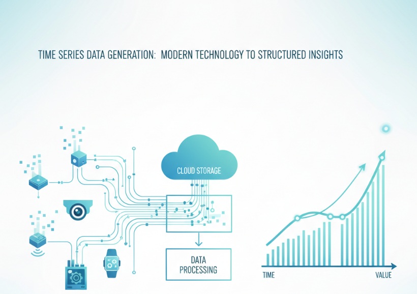Figure 3. Origin of time-series data and structure insights (the figure is generated by Artlist.io).

The analysis of time series data is therefore essential in almost every scientific discipline and industrial domain. However, the inherent complexity of the underlying data-generating systems, combined with measurement errors and the influence of external factors, often leads to irregular phenomena. These irregular events subsequently appear in the collected data as anomalies. By anomalies, we refer to data points or groups of data points that do not conform to a certain notion of normality or expected behavior derived from previously observed data.

Time series anomaly detection has received sustained attention in both academia and industry for more than six decades. Depending on the application, anomalies can be categorized as:
1. Noise or erroneous data that hinders downstream analysis;
2. Data of genuine interest that should be retained and investigated.

In the first case, anomalies are considered undesirable and are removed or corrected. In the second case, anomalies may indicate meaningful events, such as failures or changes in behavior, which form the basis for further analysis.

Consequently, detecting anomalies in time series yields substantial benefits, especially in real-world systems such as IoT, finance, manufacturing, and healthcare.

First, anomaly detection enables early identification of warning signs before severe incidents occur. For example, when a server experiences a sudden surge in traffic, an anomaly detection system can raise alerts about potential attacks or system failures. Early detection in such scenarios helps reduce downtime and associated repair costs.

Second, from a maintenance perspective, detecting anomalous points helps operators avoid unnecessary maintenance operations.

A particularly important practical application of anomaly detection lies in fraud detection for banking and e-commerce transactions.

Figure 4. Early anomaly detection prevents unexpected circurstances (the figure is genetrated by ChatGPT).

To identify anomalous points, several categories of methods have been studied:

• Methods that introduce a transformation step to map temporal information into a suitable vector space, followed by the application of traditional machine learning–based outlier detection techniques such as XGBoost, Decision Trees, and others.

• Methods that employ specialized distance or similarity measures for time series in order to identify anomalous time series or anomalous subsequences.

• Methods from the deep learning community that leverage specialized architectures capable of encoding temporal information, such as recurrent neural networks (RNNs) or convolution-based approaches.

Types of Anomalies

Due to the temporal dependence intrinsic to the data, anomalies may appear as individual points or as subsequences. In the case of point anomalies, the goal is to identify data points that lie far from the typical value distribution representing normal operating conditions. By contrast, in sequence anomalies, the objective is to detect anomalous subsequences; these subsequences are not necessarily composed of individual outliers, but instead exhibit rare patterns and are therefore considered anomalous. In practical applications, distinguishing between point anomalies and sequence anomalies is particularly important, since a single data point may appear normal relative to its neighbors, whereas the overall shape of the corresponding subsequence may still indicate abnormal behavior.

Formally, anomalies in time series can be categorized into three principal types: point anomalies, contextual anomalies, and collective anomalies.

• Point anomalies are individual data points whose values deviate significantly from the rest of the dataset. In this case, the anomalous value lies outside the expected range of normal behavior.

• Contextual anomalies are data points that remain within the global value distribution (unlike point anomalies) but deviate from the expected behavior when considered within a specific context, such as a local time window.

• Collective anomalies are groups of data points forming subsequences that do not conform to typical patterns observed in the data, and thus exhibit abnormal structure or behavior at the sequence level.

The first two types, namely point anomalies and contextual anomalies, are often jointly referred to as point-based anomalies, whereas collective anomalies are categorized as sequence-based anomalies.

In addition, another variant of subsequence anomaly detection, known as whole-sequence detection, should be distinguished from point-wise detection. In this setting, the subsequence spans the entire time series, and the whole series is treated as a single entity for anomaly assessment.

This approach frequently arises in sensor data cleaning tasks, where researchers aim to identify malfunctioning sensors among a set of otherwise normally operating sensors.

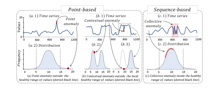Figure 5. Classification of anmalies in time series data [1].

Distance-Based Methods for Detecting Anomalies

Distance-based methods identify anomalous points in time series data based on the distances between data points (for example, Euclidean distance).

Representative models in this family can be grouped into three main categories:

Proximity-based Methods

Methods in this group treat a sub-sequence in a time series as a data point in a multi-dimensional space, and a data point is considered anomalous if it is significantly isolated from its nearest neighbors.

Representative models:
- Kth Nearest Neighbor (KNN)
- Local Outlier Factor (LOF)

Clustering-based Methods

These methods partition sub-sequences of the time series into different clusters. A data point is classified as anomalous if it does not belong to any cluster or lies too far from the centroid of the nearest cluster.

Representative models:
- K-means
- DBSCAN
- MCOD

Discord-based Methods

This approach searches for discords—subsequences that have the largest distance to their nearest neighboring subsequences, compared to all others.

Representative models:
- Matrix Profile
- HOT SAX
- DAD

Strengths and Weaknesses

Distance-based methods typically preserve the original form of the time-series data, avoiding transformations or feature augmentations, and are relatively easy to implement. However, when anomalous points form small, dense clusters, traditional techniques such as KNN may struggle to identify them accurately.

Application Scenarios

These approaches are especially effective for unsupervised learning problems, where training data are unlabeled or where the task is to detect outliers that lie outside the distribution of the training data.

Density-based Methods

Density-based methods transform time-series data into more complex data structures to measure the density of data points or subsequences.

Distribution-based Methods

These methods use statistical characteristics of normal subsequences (e.g., variance, standard deviation) to construct a probabilistic model of normality, which helps distinguish anomalous data points.

Representative models:
- Minimum Covariance Determinant (MCD)
- One-Class SVM (OCSVM)
- Histogram-based Outlier Score (HBOS)

Graph-based Methods

In this group, the time series is represented as a graph, where nodes correspond to subsequences and edges capture the transition frequencies between them. Anomalies are detected through graph properties such as irregular paths, low node degrees, or weak edge weights.

Representative models:
- Finite State Machine (FSM)
- Series2Graph

Tree-based Methods

These methods employ tree-structured data representations to segment data. Anomalies correspond to isolated nodes (typically at shallow depths) that deviate from the overall data distribution.

Representative models:
- Isolation Forest (IForest)

Encoding-based Methods

In encoding-based approaches, time-series data are encoded or compressed into discrete symbols. A data point is deemed anomalous depending on how well the encoded representation matches the new observed data.

Representative models:
- Principal Component Analysis (PCA)
- GrammarViz
- Hidden Markov Model (HMM)
- Dynamic Bayesian Network (DBN)

Strengths and Weaknesses

Density-based methods are particularly effective in capturing complex, cyclic, or topological structures rather than focusing solely on individual data points. However, they may involve computationally intensive preprocessing steps or require precise data representations.

Application Scenarios

These methods perform well on noisy and multivariate time-series data, and are widely applied in semi-supervised settings.

Prediction-based Methods

Prediction-based approaches aim to detect anomalies by predicting expected normal behaviors using a training set of time series or subsequences (which may or may not contain anomalies).

For example, when monitoring stock prices of companies such as PNJ or FPT, price fluctuations that deviate drastically from the overall trend represent the signals that these methods are designed to capture.

To address this problem, prediction-based approaches are among the most powerful strategies. They are generally divided into two levels: forecasting-based and reconstruction-based methods. All related techniques are summarized in Table 3 below.

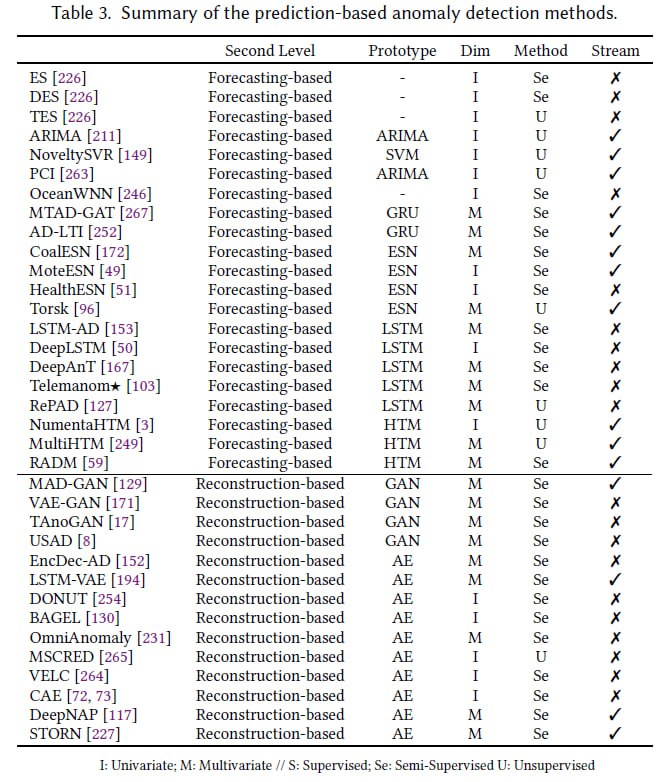
Forecasting-based Methods

Forecasting-based methods rely on a fundamental principle: using past data points or subsequences to train a model that predicts future values. The predicted results are directly associated with prior observations within the time series. Each observed data point is then compared with the corresponding predicted value—the larger the deviation (prediction error), the higher the likelihood that the point is anomalous.

Exponential Smoothing

Principle: Exponential Smoothing is among the earliest forecasting techniques proposed in the academic literature. It is a nonlinear smoothing method that predicts new data points using past observations while assigning exponentially decreasing weights to older data.

Mathematically, the estimated value at the current time step is a linear combination of previous data points. The parameter $\alpha \in [0,1]$ denotes the smoothing factor; smaller values of $\alpha$ give greater influence to older observations.

The predicted value at time $i$, denoted as $\hat{T}_i$, is calculated as follows:

$$ \hat{T}_i = (1-\alpha)^{N-1}T_{i-N} + \sum_{j=1}^{N-1}\alpha(1-\alpha)^{j-1}T_{i-j}, \quad \alpha \in [0,1] $$

Representative variants:
- Double Exponential Smoothing (DES): Designed for non-stationary time series, it introduces an additional parameter to smooth the trend component of the data.
- Triple Exponential Smoothing (TES): Similar to DES but further incorporates a third parameter to explicitly model seasonality.

Other Forecasting-based Methods

In principle, any regression model capable of predicting future values from historical data can serve as the forecasting core. Several specific architectures that have been employed include:
- OceanWNN: Utilizes Wavelet Neural Networks (Wavelet-Neural Networks).
- NoveltySVR: Relies on classical regression techniques, in particular Support Vector Regression (SVR), where the Support Vector Machine acts as the core forecasting unit.

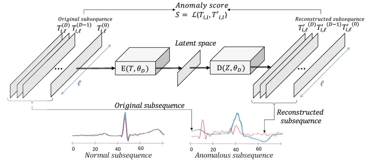Figure 6. Classification of anmalies in time series data [1].

Reconstruction-based Methods

Reconstruction-based methods represent normal behavior by encoding sub-sequences of a normal training time series into a low-dimensional space. These sub-sequences are then reconstructed (decoded) from this low-dimensional space and directly compared with their original counterparts. The difference between the reconstructed and original sequence, referred to as the reconstruction error, is used to detect anomalies. In general, the inputs to this reconstruction process are training sub-sequences extracted from the training dataset.

Autoencoder

Principle of operation:
An autoencoder is a type of artificial neural network designed to learn to reconstruct its input data through a compressed encoding whose dimensionality is smaller than that of the original input, thereby preventing the network from simply learning the identity mapping. As a core idea, the autoencoder aims to learn a latent representation that best describes the data by minimizing a reconstruction loss. Consequently, it learns to compress the dataset into a short code and then decompress that code back into data that matches the original input as closely as possible.

Formally, given two mapping functions (E) and (D) (corresponding to the encoder and decoder), the task of an autoencoder can be expressed as:

$$ \begin{aligned} \phi &: \mathbb{T}_\ell \rightarrow \mathbb{Z} \\ \psi &: \mathbb{Z} \rightarrow \mathbb{T}_\ell \\ \phi, \psi &= \arg \min_{\phi, \psi} \mathcal{L}\big(T_{i,\ell}, \psi(\phi(T_{i,\ell}))\big) \end{aligned} $$

Here, $\mathcal{L}$ denotes the loss function, which is typically chosen as the Mean Squared Error (MSE) between the input data and its reconstruction:

$$ \|T_{i,\ell} - \psi(\phi(T_{i,\ell}))\|^2 $$
This loss is particularly suitable for sub-sequences of time series, as it directly corresponds to the Euclidean distance between the original and reconstructed signals.

The reconstruction error serves as an anomaly score in anomaly detection. Since the autoencoder is trained only on normal sub-sequences (without anomalies), it is optimized to reconstruct “healthy” patterns well. Therefore, sub-sequences that deviate from the training distribution will generally yield higher reconstruction errors.

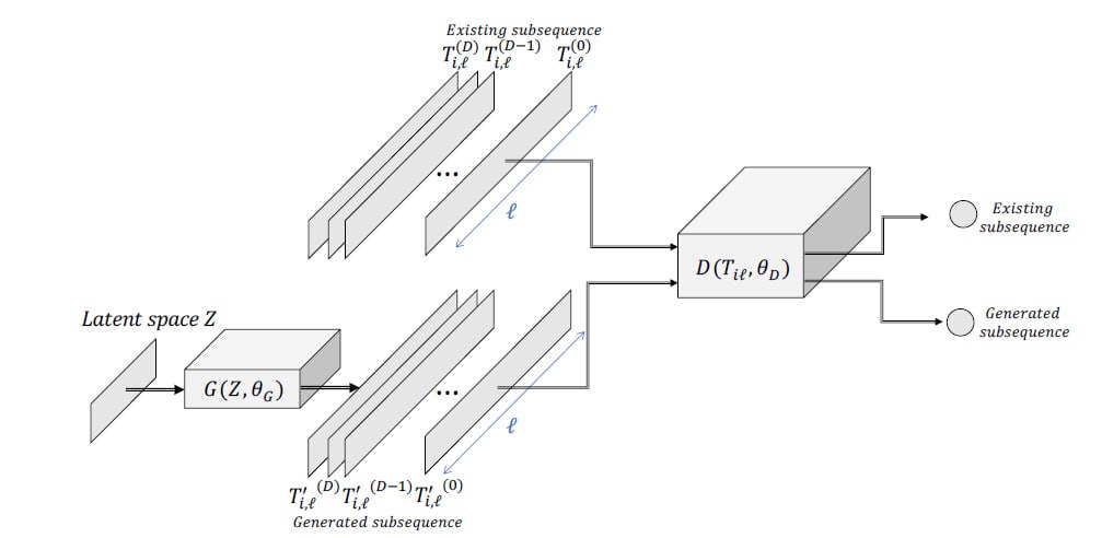Figure 7. Classification of anmalies in time series data [1].

Representative variants / frameworks:

• EncDec-AD: One of the earliest models to leverage an encoder–decoder architecture and reconstruction error to quantify abnormality.
• LSTM-VAE and MSCRED: Integrate memory mechanisms such as LSTM and Convolutional LSTM into the autoencoder architecture to better exploit temporal information.
• OmniAnomaly: An autoencoder-based method that uses GRU networks combined with planar normalizing flows to model complex data distributions.
• STORN and DONUT: Both employ Variational Autoencoders (VAEs) for anomaly detection. DONUT additionally introduces preprocessing to handle missing data via MCMC-based imputation.
• BAGEL: An improved variant of DONUT that uses a conditional VAE architecture instead of a standard VAE.
• VELC: Imposes additional constraints on the VAE, where the decoder is regularized using available anomalous samples to limit its ability to reconstruct anomalous data well.
• CAE (Convolutional Autoencoder): Uses convolutional networks to map time series to an image-like representation, and exploits SAX (Symbolic Aggregate approXimation) to accelerate search over embedded representations.
• DeepNAP: A sequence-to-sequence autoencoder model with pre-detection capability that allows anomalies to be detected before they actually occur.

Generative Adversarial Networks (GAN)

Principle of operation:
Generative Adversarial Networks (GANs) were originally introduced for image generation, but their architecture can also be adapted to generate time-series data. A GAN consists of two key components: (i) a module that generates synthetic time series, and (ii) a module that discriminates between real and generated time series. Both components play crucial roles in anomaly detection.

More concretely, a GAN involves two neural networks trained in an adversarial manner. The first is the Generator $(G(z,\theta_{g}))$, parameterized by $(\theta_{g})$. The second is the Discriminator $(D(x,\theta_{d}))$, parameterized by $(\theta_{d})$. The output of the Discriminator is a scalar value representing the probability that the input sample originates from the real dataset. Training these two networks is formulated as a two-player optimization problem: the Discriminator attempts to maximize its classification accuracy, while the Generator tries to minimize it by producing synthetic data that are indistinguishable from real data.

For anomaly detection, the Generator is trained to generate only sub-sequences labeled as “normal”, whereas the Discriminator learns to clearly separate real (normal) data from generated (abnormal) data. Consequently, both components can be exploited for anomaly detection:
- Since the Discriminator is trained to distinguish real from fake data, it can be directly used as an anomaly detector.
- The Generator is equally important. Because it is trained to generate normal sub-sequences, it tends to produce large errors when attempting to reconstruct anomalous sequences. Thus, the Euclidean distance between a target sub-sequence and the Generator’s output provides a crucial signal for determining the anomaly score.

Representative variants / frameworks:

• MAD-GAN, USAD, and TAnoGAN: These methods train GAN architectures on normal segments of the time series. The anomaly score is derived from a combination of discriminator loss and reconstruction loss.
• VAE-GAN: Combines the strengths of GANs and VAEs by designing the Generator as a VAE that competes with the Discriminator. The anomaly score is computed in a manner similar to MAD-GAN and USAD.

Conclusions

In this survey, we have provided a comprehensive overview of anomaly detection in time series. We began by constructing a detailed taxonomy of time-series types, anomaly types, and detection methods. These methods were organized into process-centric categories, and for each group we described the most widely used algorithms and compiled an extended list of existing approaches. Finally, we discussed benchmarking in depth, listing standard datasets, traditional evaluation metrics and their limitations, as well as recent efforts to adapt these metrics to the specific characteristics of time-series anomalies.

Current Challenges

Despite several decades of research, time-series anomaly detection remains highly challenging. Historically, research communities have tended to approach the problem in a fragmented way, developing methods grounded in distinct theoretical foundations. The lack of unified evaluation metrics and shared benchmark datasets has made it difficult to reliably quantify progress. Nevertheless, recent initiatives to construct benchmark collections \cite{113, 185} have significantly contributed to assessing methodological advances and selecting suitable techniques for specific application scenarios.

Future Research Directions

Although substantial progress has been made, there are still many promising directions for future research:

• Unified benchmarking: There is still no consensus on a common benchmark suite for the entire community. Existing datasets remain limited in terms of time-series diversity, anomaly types, and label reliability. Developing a more standardized and comprehensive evaluation framework is therefore crucial.
• Model selection and AutoML: With new methods being introduced every year, recent studies indicate that no single model is universally optimal across all datasets. This motivates approaches based on model ensembling, model selection, and AutoML. Empirical results suggest that leveraging basic time-series classification models to assist in selecting anomaly detection models can substantially improve accuracy, in some cases by up to a factor of two.
• Extension to complex data scenarios: Most unsupervised methods currently focus on univariate time series, whereas real-world applications are often far more complex. Future work needs to address settings such as multivariate time series, streaming data, missing values, irregular time stamps, heterogeneous data sources, and combinations thereof. Developing robust and accurate methods for these challenging scenarios remains an urgent and important research goal.

[1] Boniol, P., Liu, Q., Huang, M., Palpanas, T., & Paparrizos, J. (2024). Dive into time-series anomaly detection: A decade review. arXiv. https://arxiv.org/abs/2412.20512