PROJECT WARMUP PHASE 1: EMPLOYEE ATTRITION RISK PREDICTION
Proposed Models: Random Forest and Logistic Regression
PART 1. OVERVIEW AND PROBLEM STATEMENT
1.1. Problem Statement
Employee turnover incurs significant costs for businesses. Rather than reacting passively, this project builds an early warning tool for attrition risk prediction based on historical data, helping managers proactively develop strategies to retain talent.
1.2. Proposed Solution
Develop a Web application (Streamlit) integrated with Machine Learning models (Random Forest & Logistic Regression). The system is optimized with only 7 core input indicators (Salary, OT, Age...), enabling fast and accurate predictions.
1.3. Technical Challenges
- Imbalanced Data: The actual attrition rate is very low (16.1%). The team used SMOTE technique to generate synthetic data, helping the model avoid majority class bias.
- Trade-off between Accuracy and Usability: Entering 35 fields of information is overwhelming for users. The team performed Feature Selection to choose the 7 most important variables, ensuring the application is lightweight while maintaining high prediction performance.
PART 2. IMPLEMENTATION PROCESS
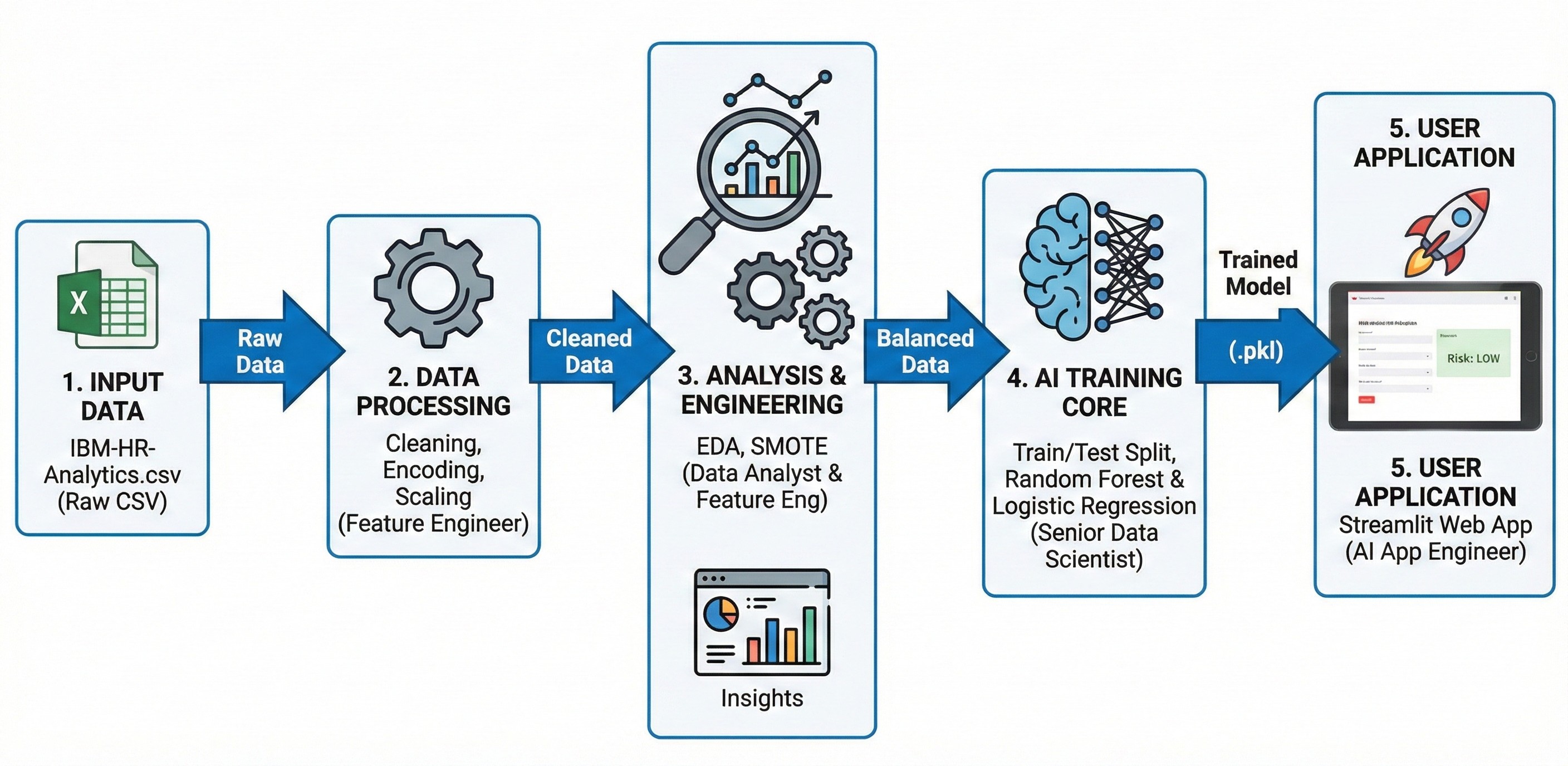
Figure 1: Overall pipeline for the project
2.1. Data Initialization and Preparation
-
Data source: IBM HR Analytics Employee Attrition & Performance sample dataset (CSV format) containing aggregated employee records, including demographic information, salary levels and work history of 1,470 employees (with 35 characteristic attributes).
-
Read data using pandas, pd.read_csv() function is used to load data from the source file into memory (DataFrame) for analysis.
# Đọc dữ liệu
df = pd.read_csv(CSV_PATH)
print(f"✅ Đọc thành công {len(df)} records từ CSV")
print(f"\n📊 Shape: {df.shape}")
print(f"📊 Columns: {df.shape[1]} columns")
✅ Đọc thành công 1470 records từ CSV

📊 Shape: (1470, 35)
📊 Columns: 35 columns
2.2. Exploratory Data Analysis (EDA) and Feature Selection
Before inputting into the model, the team performed exploratory analysis on all 35 attributes and drew important conclusions:
- Imbalanced Data: The target variable
Attritiondistribution is highly skewed: 16.1% Leave (Yes) vs 83.9% Stay (No).
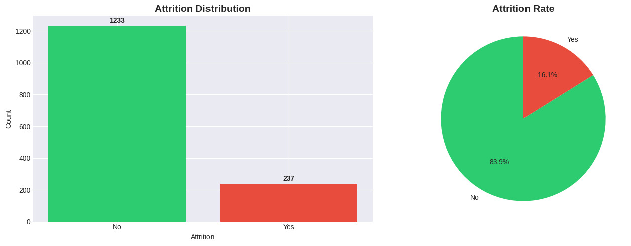
Figure 2: Attrition distribution.
-
Key Drivers:
-
OverTime: Employees who work overtime (Yes) have a significantly higher attrition rate (~3 times higher than those who don't).
-
MonthlyIncome: The Boxplot shows that the group who left has a significantly lower median salary compared to those who stayed.
-
Age & Tenure: Young employees (under 30 years old) and those with low tenure (low TotalWorkingYears) tend to have the highest job-hopping rate.
-
MaritalStatus: Single employees have a higher attrition rate than married or divorced employees.
-
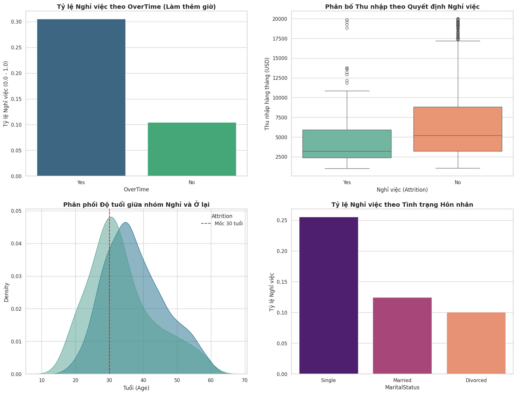
Figure 3: Analysis of key factors affecting attrition decision (Attrition Drivers). Results show that OverTime, Low Income, Young Age, and Single status are the top causes.
-
Correlation Analysis:
-
Detected strong multicollinearity (~0.95) between MonthlyIncome and JobLevel.
-
Decision: Remove JobLevel and keep MonthlyIncome because continuous variables provide more detailed information.
-
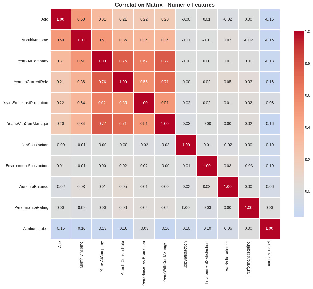
Figure 4: Correlation matrix between variables.
2.3. Data Preprocessing
Based on EDA results, the preprocessing process was performed in 5 steps:
- Feature Selection:
- To optimize model performance and user experience in the application, the team reduced from 35 attributes to 7 core attributes:
OverTime,MonthlyIncome,Age,TotalWorkingYears,YearsAtCompany,JobSatisfaction,MaritalStatus.
selected_columns = [
        'Attrition',           # Target
        'OverTime',            # Feature 1
        'MonthlyIncome',       # Feature 2
        'Age',                 # Feature 3
        'TotalWorkingYears',   # Feature 4
        'YearsAtCompany',      # Feature 5
        'JobSatisfaction',     # Feature 6
        'MaritalStatus'        # Feature 7
    ]

df = df[selected_columns]
- Feature Encoding:
- Binary Encoding: Convert Attrition (Yes/No) $\rightarrow$ (1/0); OverTime (Yes/No) $\rightarrow$ (1/0).
df['Attrition'] = df['Attrition'].apply(lambda x: 1 if x == 'Yes' else 0)
df['OverTime'] = df['OverTime'].apply(lambda x: 1 if x == 'Yes' else 0)
- One-Hot Encoding: Applied to the categorical variable MaritalStatus. Use drop_first=True parameter to avoid the Dummy Variable Trap, keeping only _Married and _Single columns (if both are 0, it means Divorced).
df_reduce = pd.get_dummies(df_reduce, columns=['MaritalStatus'], drop_first=True)
- Data Splitting:
-
Ratio: 80% Train (1176) - 20% Test (294).
-
Use stratify=y to ensure the attrition rate in both sets is equivalent.
X_train, X_test, y_train, y_test = train_test_split(X, y, test_size=0.2, random_state=42, stratify=y)
- Feature Scaling:
Use StandardScaler to bring numerical variables (Age, MonthlyIncome, TotalWorkingYears, YearsAtCompany, JobSatisfaction) to the same standard distribution.
numeric_cols = ['Age', 'MonthlyIncome', 'TotalWorkingYears', 'YearsAtCompany', 'JobSatisfaction']
scaler = StandardScaler()

X_train[numeric_cols] = scaler.fit_transform(X_train[numeric_cols])
X_test[numeric_cols] = scaler.transform(X_test[numeric_cols])
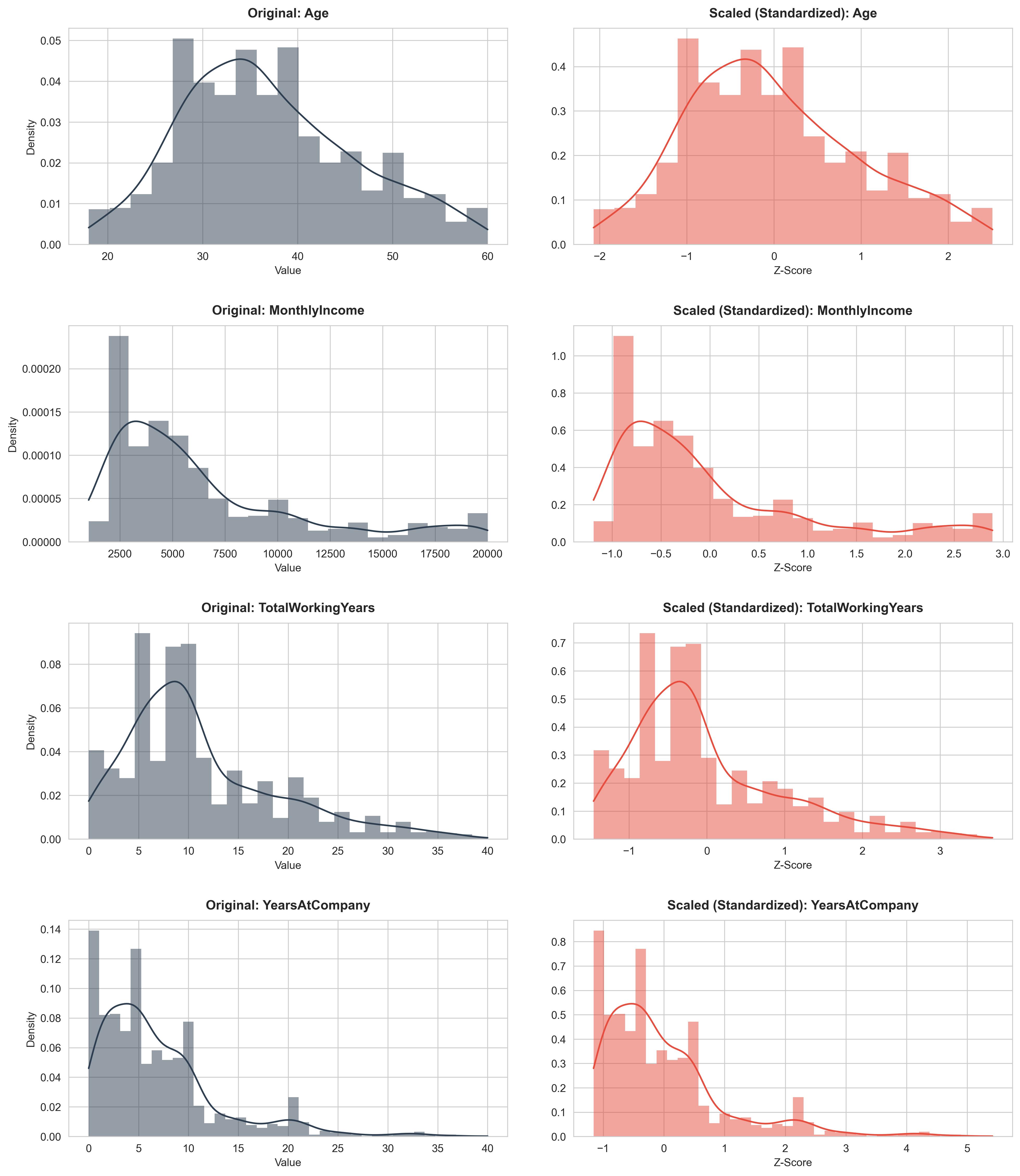
Figure 5: Before and after data scaling.
- Imbalance Handling:
The initial training set was severely skewed toward the "Stay" employee class (Class 0), making the model prone to missing "Leave" employee cases (Class 1). The team used the SMOTE algorithm to generate additional synthetic data for the minority class based on the k-Nearest Neighbors (k-NN) principle in the standardized vector space. The result is that the number of samples in both classes becomes balanced (50/50), helping the model learn the characteristics of the leaving group better and avoiding bias toward the majority group.
smote = SMOTE(random_state=42)
X_train_resampled, y_train_resampled = smote.fit_resample(X_train, y_train)
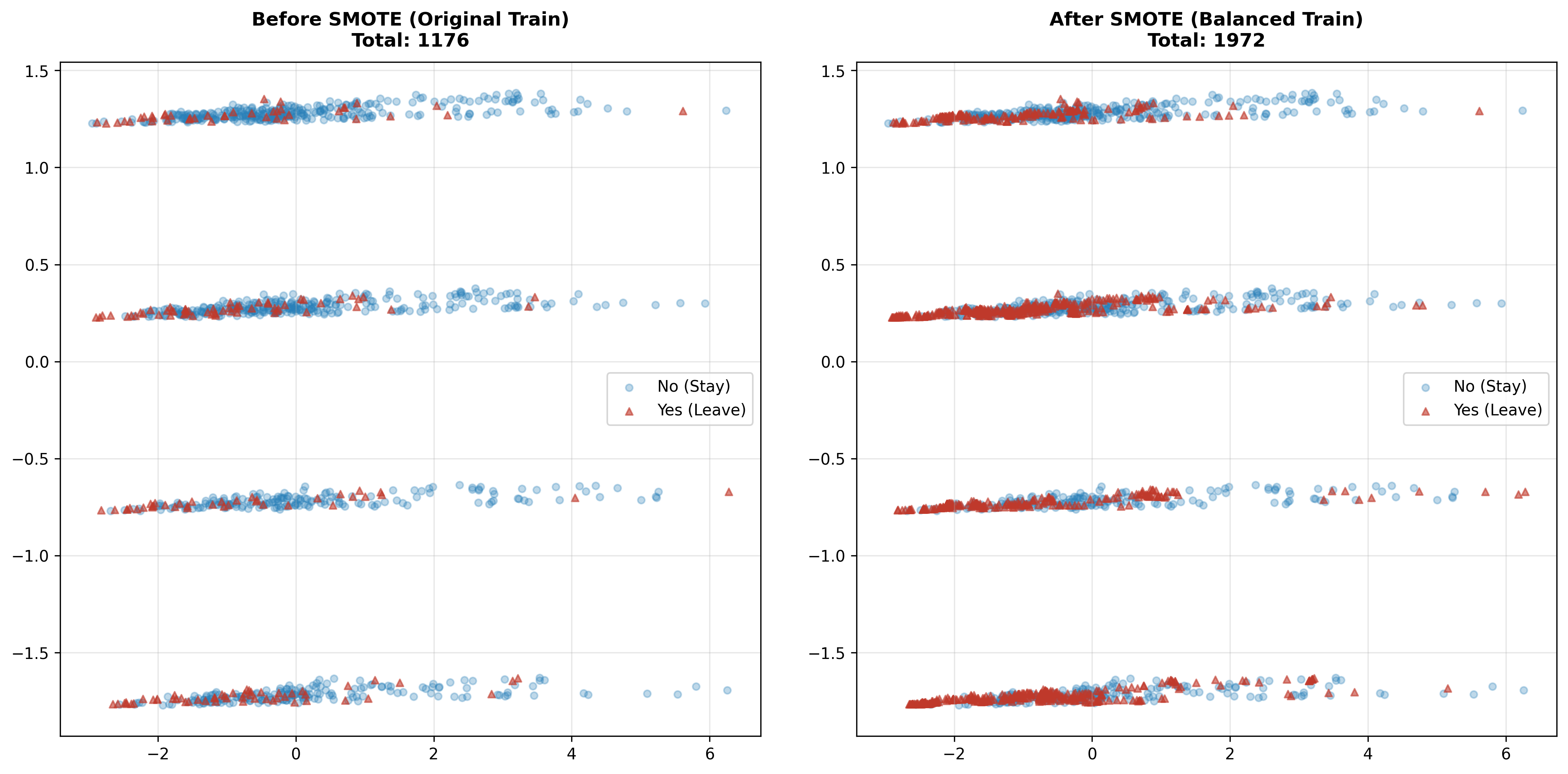
Figure 6: Before and after adding data.
2. Data Description
After the selection process, the final dataset used for training includes the following 8 columns:
| No. | Attribute Name | Data Type | Role | Detailed Description |
|---|---|---|---|---|
| 1 | Attrition | Binary (0/1) | Target | Target variable: 1 is Leave (Yes), 0 is Stay (No). |
| 2 | OverTime | Binary (0/1) | Feature | Does the employee work overtime? (This is the strongest factor affecting attrition decision). |
| 3 | MonthlyIncome | Numerical (Int) | Feature | Monthly income (USD). Reflects financial motivation. |
| 4 | TotalWorkingYears | Numerical (Int) | Feature | Total years of work experience (including at previous companies). |
| 5 | YearsAtCompany | Numerical (Int) | Feature | Years of tenure at current company. |
| 6 | JobSatisfaction | Ordinal (1-4) | Feature | Level of satisfaction with current job. Scale: 1 (Low) to 4 (Very High). |
| 7 | MaritalStatus | Nominal | Feature | Marital status (Single/Married/Divorced). Single group tends to have higher attrition probability. |
PART 3. MODEL TRAINING AND EVALUATION
After completing data preprocessing, the team proceeded to train two popular machine learning models: Logistic Regression and Random Forest. These are two algorithms representing two different approaches: linear and non-linear/ensemble, providing a multi-dimensional view of prediction capability.
3.1. Model Selection and Configuration
3.1.1. Logistic Regression
Reasons for selection:
-
It is a fundamental algorithm for Binary Classification problems.
-
Easy to interpret: Model weights indicate the positive or negative influence of each feature on attrition probability.
-
Computationally efficient: Short training time, suitable for datasets of moderate size like this project.
Configuration:
from sklearn.linear_model import LogisticRegression

lr_model = LogisticRegression(random_state=42, max_iter=1000)
lr_model.fit(X_train_resampled, y_train_resampled)
-
random_state=42: Ensures reproducibility.
-
max_iter=1000: Maximum number of iterations for convergence.
3.1.2. Random Forest
Reasons for selection:
-
Is an ensemble model based on multiple decision trees, capable of capturing complex non-linear relationships in data.
-
Resistant to overfitting thanks to the bagging mechanism and random feature selection.
-
Provides feature importance, helping to understand the contribution of each variable.
Configuration:
from sklearn.ensemble import RandomForestClassifier

rf_model = RandomForestClassifier(
    n_estimators=100,
    max_depth=10,
    min_samples_split=10,
    random_state=42
)
rf_model.fit(X_train_resampled, y_train_resampled)
-
n_estimators=100: Number of decision trees in the forest.
-
max_depth=10: Maximum depth of each tree (helps prevent overfitting).
-
min_samples_split=10: Minimum number of samples required to split a node.
3.2. Model Evaluation
3.2.1. Evaluation Metrics
Due to the imbalanced data nature, overall Accuracy alone is not sufficient. The team used the following metrics:
-
Precision: Ratio of correct predictions among cases predicted as "Leave". Reflects False Positive risk (mistakenly warning about loyal employees).
-
Recall (Sensitivity): Ratio of actual "Leave" cases correctly detected. This is the most important metric because it directly impacts the goal of early attrition detection.
-
F1-Score: Harmonic mean of Precision and Recall, providing balanced evaluation.
-
AUC-ROC: Area under the ROC curve, measuring the model's ability to rank risk probabilities.
3.2.2. Classification Report
Below is a detailed comparison of the two models on the Test set (294 samples):
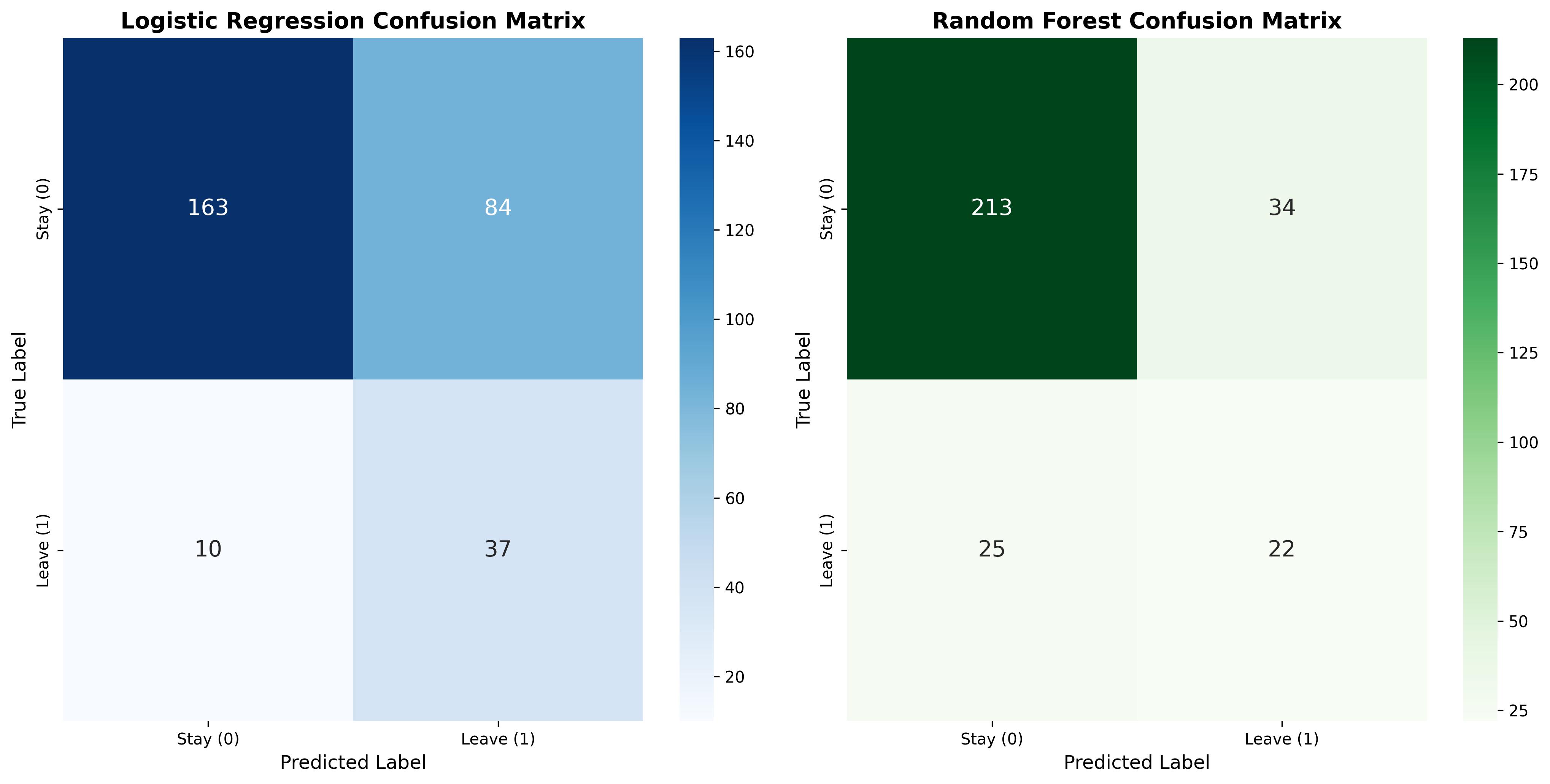
Figure 7: Compare the Confusion Matrix on the test set.
Logistic Regression Accuracy: 0.6837
              precision    recall  f1-score   support

           0       0.87      0.66      0.75       247
           1       0.23      0.53      0.32        47

    accuracy                           0.68       294
   macro avg       0.62      0.72      0.61       294
weighted avg       0.84      0.68      0.72       294

Random Forest Accuracy: 0.7993
              precision    recall  f1-score   support

           0       0.89      0.86      0.88       247
           1       0.39      0.47      0.43        47

    accuracy                           0.80       294
   macro avg       0.64      0.67      0.65       294
weighted avg       0.81      0.80      0.81       294
Based on experimental results, important findings were drawn:
- Logistic Regression:
-
Strength: Recall for the Leave class reached 79% (correctly detected 37/47 cases). This is the biggest advantage, helping businesses not miss personnel who intend to leave.
-
Limitation: Low overall accuracy (68%) due to too high False Positive rate. Up to 84 loyal employees were mistakenly predicted to leave.
- Random Forest:
-
Strength: Very high overall Accuracy, reaching ~80%. The model operates stably with few false alarms (only 34 cases compared to 84 for Logistic).
-
Limitation: Poor risk detection capability. Recall for the Leave class only reached 47% (missed 25/47 cases), meaning more than half of employees at risk of leaving would not be warned by the system.
3.2.3. ROC Curve
To have a more objective view of the classification capability of the two models at different thresholds, the team used the ROC curve and the Area Under Curve (AUC) metric.
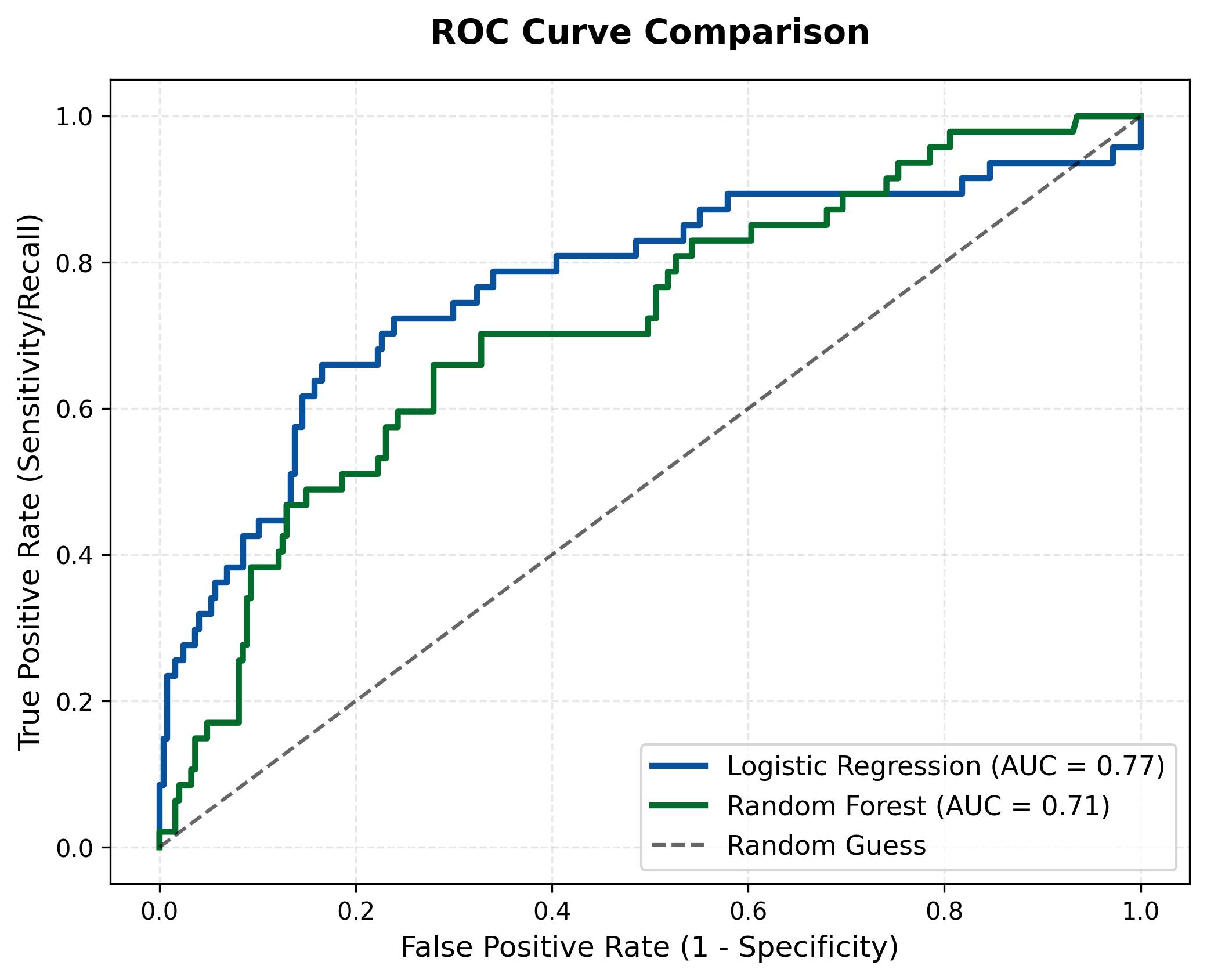
Figure 8: ROC curve comparison of two models.
Logistic Regression (Blue curve), this curve rises significantly higher and covers a larger area with an AUC of 0.77. This confirms that this linear model performs more effectively in separating the two data classes, especially in maintaining a high True Positive Rate even when accepting a low False Positive rate.
Random Forest (Green curve), the curve is lower with an AUC of only 0.71. Although it is a more complex model, Random Forest proved less effective in risk probability ranking compared to Logistic Regression in this case. Its curve tends to be closer to the random diagonal line, reflecting difficulty in clearly distinguishing cases of employees about to leave.
PART 4. APPLICATION DEPLOYMENT
4.1. Introduction to Machine Learning Model Deployment
After completing the data processing and Machine Learning model building, the next step is to deploy the model into a practical application for users to use. Deployment helps the model not only stop at the experimental level but can be applied in practice to support prediction or decision-making.
In this project, the team uses Streamlit for deployment. Streamlit is a Python framework that allows building simple and fast web interfaces for Data Science and Machine Learning applications.
4.2. Reasons for Choosing Streamlit
Streamlit was chosen due to the following advantages:
- Easy to use: Does not require deep Front-end knowledge.
- Good integration with Python: Suitable for Machine Learning models built with Python.
- Quick deployment: Just write a few lines of code to create a web interface.
- Supports visualization: Can display charts and visual analysis results.
4.3. Streamlit Application Deployment Process
4.3.1 Install necessary libraries
pip install streamlit
pip install scikit-learn
pip install pandas
pip install joblib
4.3.2 Build UI
a. User Input Section
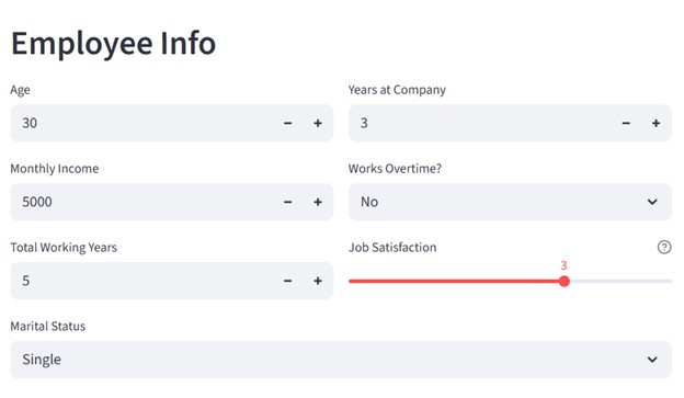
To build a UI like this, we need to divide into 2 columns:
col1, col2 = st.columns(2)
For the left column, we need to display inputs for 'age', 'Monthly Income', 'Total Working Years' variables
col1, col2 = st.columns(2)

with col1:
    age = st.number_input("Age", min_value=18, max_value=65, value=30)
    monthly_income = st.number_input("Monthly Income", min_value=1000, max_value=20000, value=5000)
    total_working_years = st.number_input("Total Working Years", min_value=0, max_value=40, value=5)
For the right column, we need to display inputs for 'Year at Company', 'Over Time', 'Job Satisfaction' variables.
with col2:
    years_at_company = st.number_input("Years at Company", min_value=0, max_value=40, value=3)
    overtime = st.selectbox("Works Overtime?", ["No", "Yes"])
    job_satisfaction = st.slider(
        "Job Satisfaction",
        min_value=1,
        max_value=4,
        value=3,
        help="1: Low, 2: Medium, 3: High, 4: Very High"
    )

marital_status = st.selectbox(
    "Marital Status",
    ["Single", "Married", "Divorced"]
)
b. Prediction Result Display UI
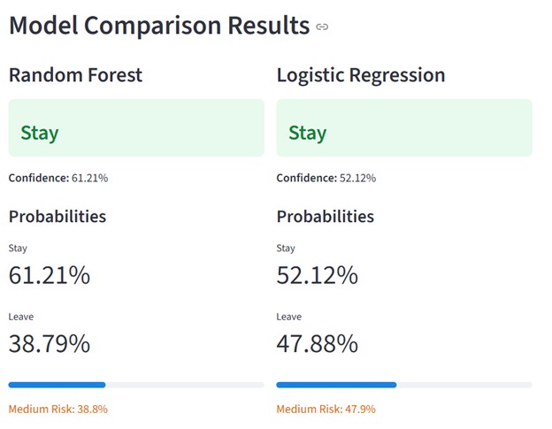
The interface is divided into two parallel columns using st.columns(2):
Column 1: Displays Random Forest model results
Column 2: Displays Logistic Regression model results
This layout helps users compare the two models visually and conveniently.
col1, col2 = st.columns(2)

with col1:
    st.subheader("Random Forest")
    if rf_prediction == 1:
        st.error(f"{rf_result}")
    else:
        st.success(f"### {rf_result}")
    st.markdown(f"**Confidence:** {rf_conf:.2f}%")

    st.markdown("#### Probabilities")
    st.metric("Stay", f"{rf_probabilities[0]*100:.2f}%")
    st.metric("Leave", f"{rf_probabilities[1]*100:.2f}%")

    st.progress(float(rf_probabilities[1]))
    leave_prob_rf = rf_probabilities[1] * 100
    if leave_prob_rf < 30:
        st.markdown(f":green[Low Risk: {leave_prob_rf:.1f}%]")
    elif leave_prob_rf < 60:
        st.markdown(f":orange[Medium Risk: {leave_prob_rf:.1f}%]")
    else:
        st.markdown(f":red[High Risk: {leave_prob_rf:.1f}%]")

with col2:
    st.subheader("Logistic Regression")
    if lr_prediction == 1:
        st.error(f"### {lr_result}")
    else:
        st.success(f"### {lr_result}")
    st.markdown(f"**Confidence:** {lr_conf:.2f}%")

    st.markdown("#### Probabilities")
    st.metric("Stay", f"{lr_probabilities[0]*100:.2f}%")
    st.metric("Leave", f"{lr_probabilities[1]*100:.2f}%")

    st.progress(float(lr_probabilities[1]))
4.4 Limitations and Future Development
Limitations
- Streamlit interface is still simple
- Limited large data processing capability
- Model performance not yet optimized
Future Development
- Optimize user interface
- Integrate multiple prediction models
- Deploy on server to serve multiple users simultaneously
- Deploy on cloud for others to try the model (Hugging Face)
References
-
Dataset IBM HR Analytics Employee Attrition & Performance - Kaggle
-
File source code - Google_Colab
Chưa có bình luận nào. Hãy là người đầu tiên!