Logistic Regression from the Start: Understanding the Gradient Through Matrices

Introduction

In modern Machine Learning courses, Logistic Regression is often dismissed as a "basic" model, even considered "boring". Many learners rush through it to jump straight into Deep Learning with more complex architectures. However, what few people realize is that the mathematics behind the Gradient of Logistic Regression is actually the solid foundation for most deep learning models today. If you don't truly understand how gradients are computed in Logistic Regression, you will struggle when trying to debug or optimize more complex models.

In this project, I decided to build Logistic Regression completely from scratch, using only NumPy — no PyTorch, no TensorFlow, no Autodiff Engine whatsoever. The goal is not to optimize performance or achieve the highest accuracy, but to understand clearly why the gradient takes the form $X^T(p - y)$, to observe the Chain Rule directly in matrix form, and to ensure no step is "hidden". This is a journey back to the roots to truly master Machine Learning from the ground up.

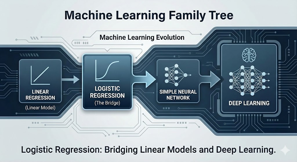
Figure 1. Logistic Regression is the bridge between Linear Model and Neural Network

I. Dataset and Data Preparation

1.1 Dataset Used

This project uses the Breast Cancer Wisconsin Dataset — a classic dataset for Binary Classification problems. This dataset contains measurements from breast cancer cell images, and the model's task is to predict whether a tumor is benign or malignant. This is a real-world medical problem where every wrong prediction can impact a patient's life.

Mathematically, we represent the dataset as follows: $X \in \mathbb{R}^{n \times d}$ is the data matrix with $n$ samples and $d$ features, while $y \in \mathbb{R}^n$ is the binary label vector (0 or 1). The reasons this dataset is suitable for the project are: binary labels match the Logistic Regression problem, all features are continuous real values suitable for linear models, and the moderate size (approximately 569 samples) makes it easy to analyze and debug when errors occur.

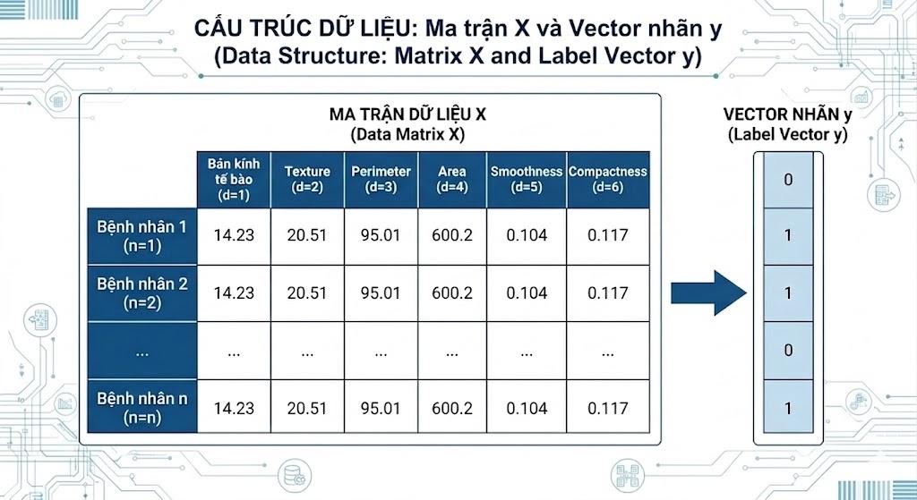
Figure 2. Illustration of data matrix X and label vector y structure

1.2 Train / Test Split

A golden rule in Machine Learning is: Never evaluate a model on data it was trained on. This is like grading your own exam — the results will be biased and won't reflect true capability. Therefore, the dataset is split into 80% training data (Training Set) and 20% testing data (Test Set).

The Training Set is used to compute gradients and update the model's Parameters. Throughout training, the model will "look at" the Training Set thousands of times to learn patterns. Conversely, the Test Set is kept as a "sealed exam room" — the model is evaluated on the Test Set only once at the end of the process, ensuring objective results and avoiding Overfitting.

1.3 Feature Scaling

Imagine you're comparing two features: "cell area" (unit: square micrometers, values from 100 to 2500) and "uniformity" (unitless, values from 0 to 1). If left as is, Gradient Descent will be dominated by the feature with larger values, making the learning process skewed and slow to converge. This is like trying to walk on a tilted surface — your steps will be pulled toward the slope instead of going straight to the destination.

To solve this problem, each feature is normalized using Standardization: $x \leftarrow \frac{x - \mu}{\sigma}$, where $\mu$ is the mean and $\sigma$ is the standard deviation. To be precise with matrix notation, this operation is applied column-wise (for each feature) across the entire data matrix X. After normalization, all features have mean = 0 and std = 1, helping Gradient Descent converge faster and more stably. An important thing to remember: normalization doesn't change the mathematical form of the gradient, it only improves numerical stability.

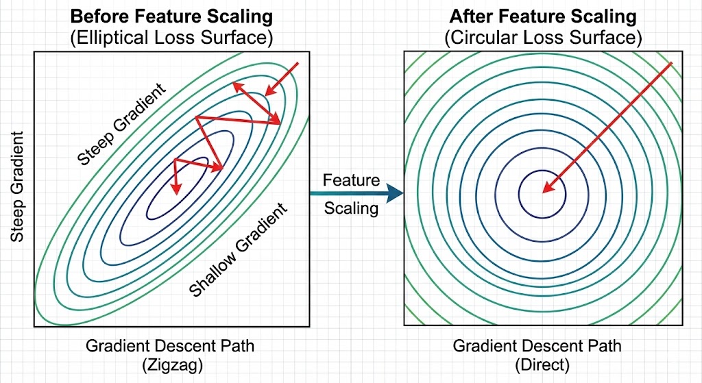
Figure 3. Comparison of Loss Surface before and after Feature Scaling

II. Model Architecture

2.1 Forward Pass

Logistic Regression operates in two sequential steps during the Forward Pass. First, we compute the Linear Combination: $z = Xw + b$, where $w \in \mathbb{R}^d$ is the weight vector and $b \in \mathbb{R}$ is the Bias. The value $z$ can be any real number from negative infinity to positive infinity, but we need probabilities within the range [0, 1].

This is where the Sigmoid Function comes in: $p = \sigma(z) = \frac{1}{1 + e^{-z}}$. This function "squashes" all real values into the range (0, 1), transforming the output into valid probabilities. When $z$ is very large (positive), $\sigma(z)$ approaches 1; when $z$ is very small (negative), $\sigma(z)$ approaches 0. The inflection point at $z = 0$ yields $\sigma(0) = 0.5$ — the natural decision threshold for binary classification problems.

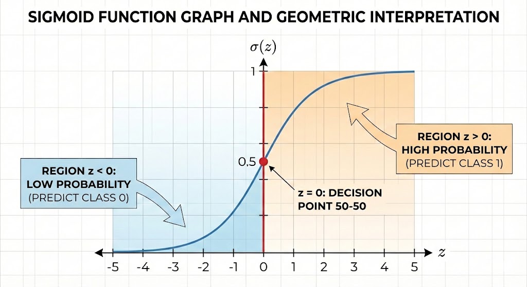
Figure 4. Sigmoid function graph and geometric meaning

2.2 The Essence of Logistic Regression

An important insight that many overlook: Logistic Regression is essentially the simplest Neural Network — a network with only 1 layer, no Hidden Layer. Input goes directly through a linear transformation, then through an activation function (Sigmoid), and produces output. If you clearly understand how gradients flow through Logistic Regression, you've already understood 80% of the Backpropagation mechanism in Deep Learning.

The only difference between Logistic Regression and a complex Neural Network is the number of layers and types of activation functions. When you stack multiple layers and replace Sigmoid with ReLU, you have a Deep Neural Network. But the principle of computing gradients — Chain Rule in matrix space — remains the same. This is why mastering Logistic Regression has long-term value.

III. Loss Function

3.1 Binary Cross-Entropy Loss

How do we measure "how wrong" the model is? We need a Loss Function — a formula that transforms the model's output and actual labels into a single number representing the "error". For binary classification problems, the most commonly used loss function is Binary Cross-Entropy (BCE):

$$L = -\frac{1}{n} \sum_{i=1}^{n} \left[ y_i \log(p_i) + (1 - y_i) \log(1 - p_i) \right]$$

Let's analyze this formula intuitively. When the actual label $y = 1$ (malignant cancer), we want $p$ to be as close to 1 as possible — in this case, $\log(p)$ will be close to 0 (low loss). Conversely, if the model predicts $p$ close to 0 while $y = 1$, $\log(p)$ will approach negative infinity (extremely high loss) — this is the penalty for wrong predictions. Similarly for the case $y = 0$. Cross-Entropy Loss "heavily penalizes" confident but wrong predictions, which is exactly the desired property.

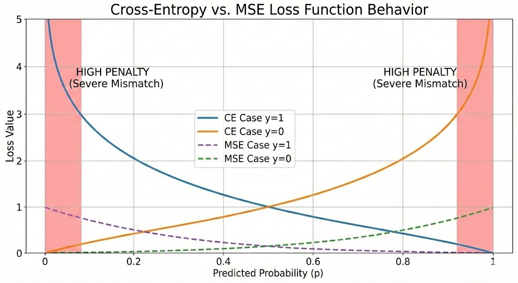
Figure 5. Cross-Entropy Loss graph versus predicted probability p

3.2 Why Loss is Always a Scalar?

A crucial point to remember: Loss is always a scalar, while parameters can be vectors or matrices. This is very important when reasoning about gradients because it shapes how we apply the Chain Rule. The gradient of Loss with respect to a parameter will have the same shape as that parameter — this is the golden rule that helps you verify the correctness of gradient formulas.

Specifically: $w \in \mathbb{R}^d$ (d-dimensional vector) → $\frac{\partial L}{\partial w} \in \mathbb{R}^d$ (also a d-dimensional vector). Similarly, $b \in \mathbb{R}$ (scalar) → $\frac{\partial L}{\partial b} \in \mathbb{R}$ (also a scalar). If the gradient you compute has a different shape than the parameter, there's definitely an error somewhere in the calculation.

IV. Parameter Initialization

4.1 Zero Initialization

In Deep Learning, initializing parameters to 0 is a taboo because it causes the Symmetry Problem — all neurons in the same layer will learn identically, causing the network to lose its representational capacity. However, Logistic Regression is an exception. Since there's only one layer and the problem is Convex, initializing $w = 0$ and $b = 0$ is perfectly safe.

Convex problems have an important property: there exists only one global minimum, and Gradient Descent will always converge to this point regardless of where it starts. There are no Local Minima or Saddle Points to get stuck in. This is one of the reasons Logistic Regression is favored in applications requiring stability and high interpretability.

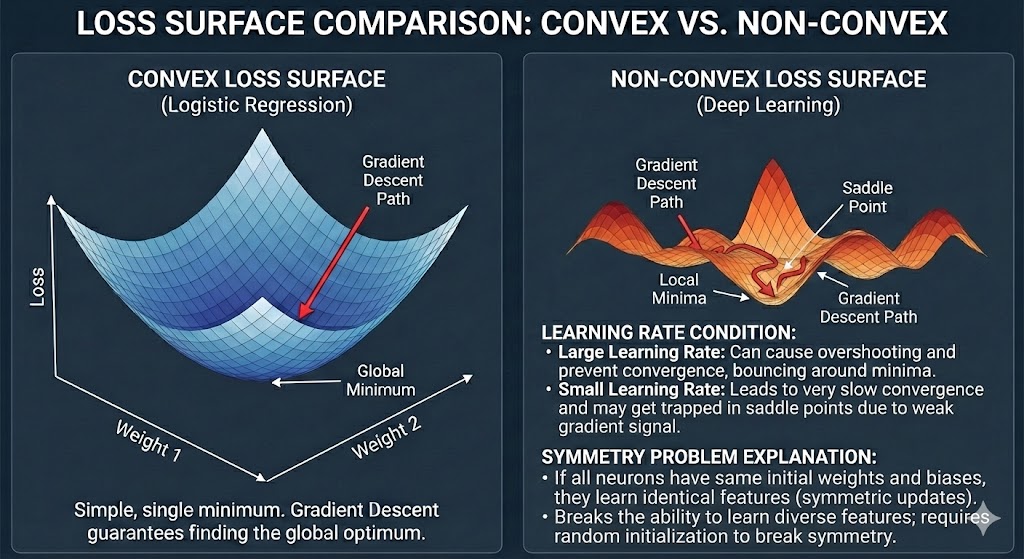
Figure 6. Comparison of Loss Surface: Convex (Logistic Regression) vs Non-Convex (Deep Learning)

V. Gradient from the Perspective of Matrix Calculus

5.1 Gradient Formula

This is the most important part of the entire project — where the Chain Rule is applied in matrix space to derive the gradient formula. After carefully applying each step (details will be presented in the code section), we obtain two elegant gradient formulas:

$$\frac{\partial L}{\partial w} = \frac{1}{n} X^T (p - y)$$

$$\frac{\partial L}{\partial b} = \frac{1}{n} \sum_{i=1}^{n} (p_i - y_i)$$

Pause and appreciate the beauty of this formula. $(p - y)$ is the Error Vector — the difference between predicted probability and actual label. $X^T(p - y)$ is the matrix multiplication of transposed $X$ with the error vector, resulting in a vector with the same shape as $w$. This is not coincidental — it's the inevitable result of the Chain Rule when applied correctly.

5.2 The Deep Meaning of $X^T(p - y)$

The expression $X^T(p - y)$ is not just a dry mathematical formula — it's the central structure that appears throughout Machine Learning. In Logistic Regression, this is the gradient of Cross-Entropy Loss. In Softmax Classifier (multi-class classification), a similar formula appears with $p$ being the softmax probability vector. In multi-layer Neural Networks, $X^T(p - y)$ is the gradient at the final layer, and previous layers are just the Chain Rule applied recursively.

If you struggle when reading papers or debugging models, come back to this formula. Understanding clearly why the gradient takes this form — from the Loss definition, through Sigmoid, to matrix multiplication — will ensure you never get "lost" in the forest of Deep Learning formulas.

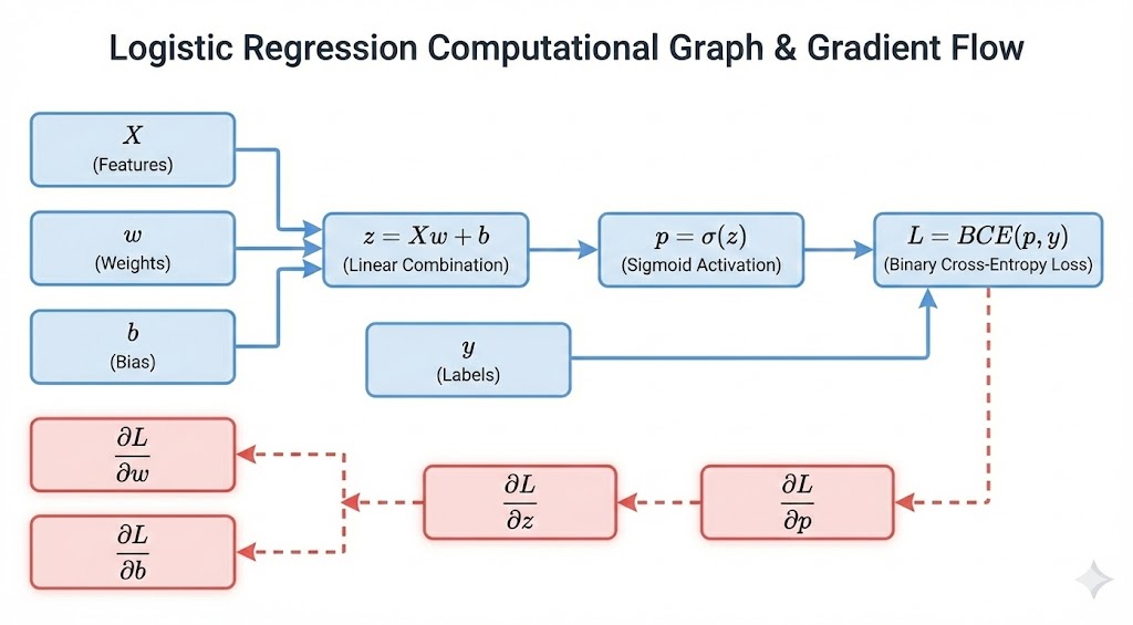
Figure 7. Computational Graph diagram of Logistic Regression

VI. Training Loop (Manual Backpropagation)

6.1 Four Steps in Each Epoch

Each Epoch consists of 4 sequential steps performed entirely manually. The first step is Forward Pass: compute $z = Xw + b$, then $p = \sigma(z)$. The second step is Compute Loss: calculate the scalar value $L$ using the Binary Cross-Entropy formula. The third step is Compute Gradient: apply the formulas $\frac{\partial L}{\partial w} = \frac{1}{n} X^T(p - y)$ and $\frac{\partial L}{\partial b} = \frac{1}{n} \sum(p - y)$. The final step is Update Parameters: $w \leftarrow w - \alpha \cdot \frac{\partial L}{\partial w}$ and $b \leftarrow b - \alpha \cdot \frac{\partial L}{\partial b}$, where $\alpha$ is the Learning Rate.

What's special about this project is that all 4 steps are coded by hand, without using PyTorch's loss.backward() or TensorFlow's tape.gradient(). Each line of code corresponds to a specific matrix operation, and you can trace exactly how gradients flow through each variable.

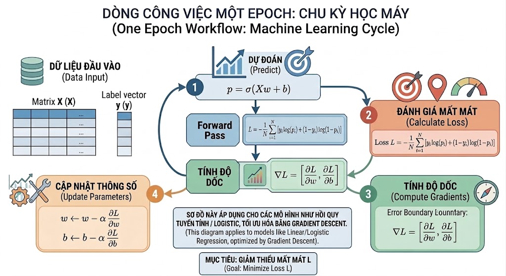
Figure 8. Flowchart of 4 steps in one Epoch

6.2 Loss Curve

After running several hundred epochs, we plot the Loss versus epoch number to check if the algorithm is working correctly. If the Loss decreases smoothly and consistently with epochs, it's a sign that: the gradient formula is correct, the learning rate is appropriately chosen, and the optimization algorithm is working properly. This is the most important way to verify gradients when doing everything from scratch.

Conversely, if the Loss fluctuates wildly (learning rate too high), Loss doesn't decrease (gradient wrong or learning rate too low), or Loss spikes then becomes NaN (numerical instability), you immediately know there's a bug to debug. The Loss curve is the "heartbeat" of the training process — always monitor it.

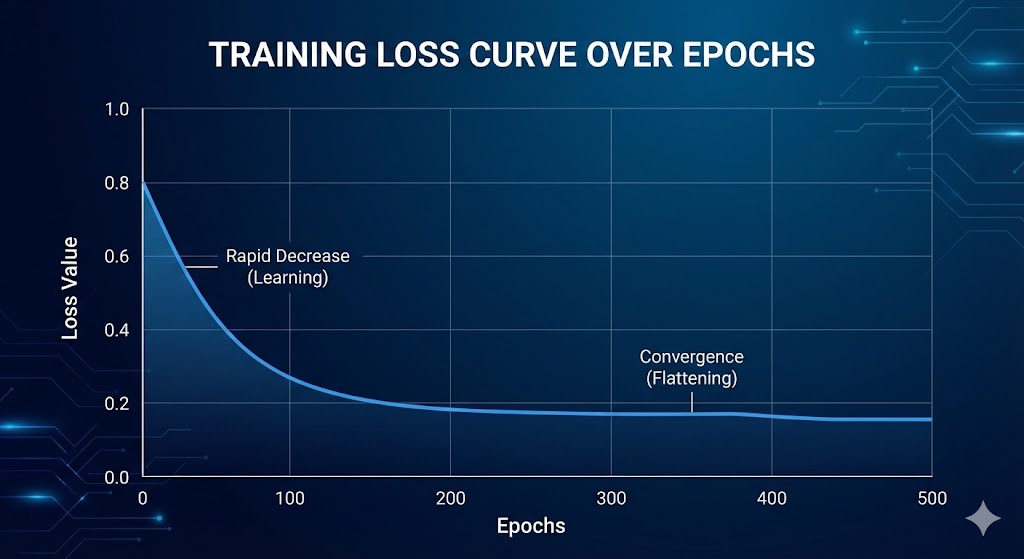
Figure 9. Loss curve decreasing over Epochs

VII. Model Evaluation

7.1 Evaluation on Test Set

After training is complete, the model is evaluated on Test data — samples it has never "seen" during the learning process. The prediction rule is very simple: if $p \geq 0.5$, predict class 1 (malignant cancer); if $p < 0.5$, predict class 0 (benign). The 0.5 threshold is the natural choice because it corresponds to the point $z = 0$ on the Sigmoid function.

Accuracy is calculated as the ratio of correctly predicted samples to total samples. With the Breast Cancer Dataset, the manually implemented Logistic Regression model achieves approximately 95-97% accuracy — equivalent to implementations using scikit-learn or PyTorch. This proves that manual implementation doesn't reduce model quality, while also showing that Logistic Regression is powerful enough for this problem.

7.2 Comparing Predictions and Ground Truth

Beyond overall accuracy, directly examining each sample is also very important. For each sample in the Test Set, we compare: predicted probability $p$, predicted label (0 or 1), and actual label (Ground Truth). This helps identify "borderline" prediction cases — samples with $p$ close to 0.5, where the model is not confident and most likely to make errors.

This detailed analysis avoids blind evaluation based solely on a single accuracy number. In medical problems, a model with 95% accuracy that often misclassifies malignant cancer as benign (False Negative) is much more dangerous than a model with 93% accuracy but errors distributed evenly on both sides. This is why Confusion Matrix, Precision, and Recall are no less important than Accuracy.

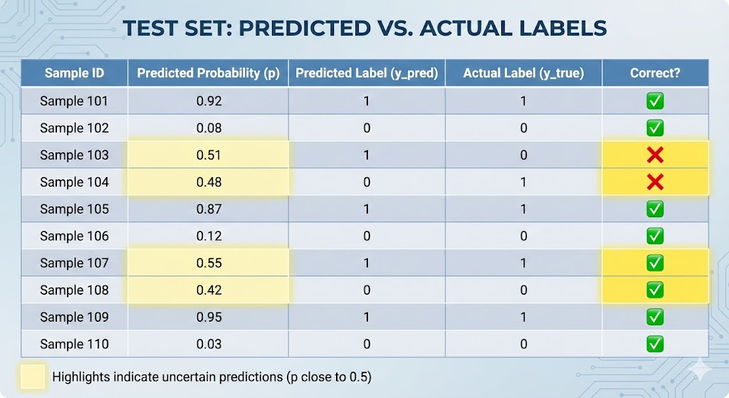
Figure 10. Comparison table of Predicted vs Actual on some Test samples

VIII. Online Demo Deployment

8.1 Gradio Web App on Hugging Face Spaces

To make the project not only academically sound but also complete in terms of application, the model is deployed as a Gradio Web App and hosted on Hugging Face Spaces. Users can directly input cell feature parameters and receive prediction probability and label (benign/malignant) within seconds. The intuitive interface allows people who don't know coding to also experience the model.

Deploying models to production is an important skill that many Machine Learning courses overlook. A model, no matter how accurate, that only exists in a Jupyter Notebook is still useless to end users. Hugging Face Spaces provides free hosting with Gradio, helping you turn a model into an actual product in just minutes.

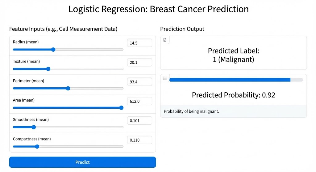
Figure 11. Gradio Web App interface for Logistic Regression

IX. Conclusion and Lessons Learned

9.1 Key Takeaways

From this project, the following important lessons can be drawn. First, Loss is always a scalar, parameters are vectors — this rule helps you verify the correctness of gradients. Second, Gradient comes from Chain Rule in matrix space — no need to write explicit Jacobians, just master the shape rules. Third, $X^T(p - y)$ is the central structure of Machine Learning — this expression appears in Logistic Regression, Softmax, and Neural Networks.

Fourth, Logistic Regression is the simplest Neural Network — understanding it clearly means you've grasped the foundation of Deep Learning. And finally, the mathematics of "basic" models is the foundation of Deep Learning — don't rush to jump to complex architectures before truly mastering the fundamentals.

9.2 Future Directions

This project opens up many natural extensions. You can implement Softmax Classifier for multi-class problems, where the gradient formula is similar but with a softmax probability vector instead of a sigmoid scalar. You can also practice Numerical Gradient Checking — a technique to verify gradients by comparing with finite differences, very useful when debugging complex formulas.

Another direction is adding L2 Regularization and deriving the gradient of the regularization term — this helps the model avoid overfitting. Finally, you can extend to 2-3 layer Neural Networks, where the Chain Rule is applied recursively through multiple layers, and you'll clearly see the same gradient pattern at every layer.

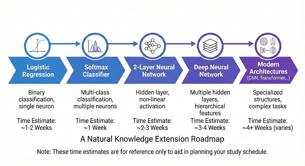
Figure 12. Roadmap from Logistic Regression to Deep Learning

Conclusion

The journey of building Logistic Regression from scratch is not just a coding exercise — it's a process of making mathematics transparent. When you manually write each line of code to compute gradients, you no longer have to "trust" autodiff as a black box. You understand why the gradient takes that form, and this understanding will stay with you throughout your Machine Learning journey, whether you work with simple or complex models.