Introduction to U-Net

Before diving into U-Net, let's explore the fundamental problem it solves

1. A Brief Look at Image Segmentation

1.1 What is Image Segmentation?

In Computer Vision, we often need to divide an image into different regions and remove redundant details to make the data easier to analyze. This process is called Image Segmentation. It focuses on identifying the location and boundaries of objects. More precisely, it is the process of assigning a label (Classification) to every pixel so that pixels belonging to the same object are grouped together.

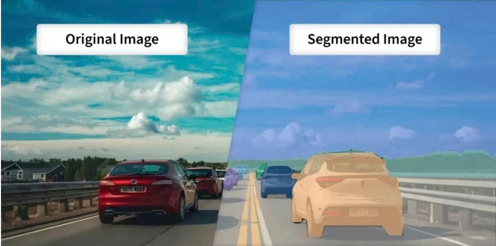
Figure 1: Original Image and Segmented Image

1.2 Classification of Image Segmentation

We can categorize Image Segmentation into three main types:

1. Semantic Segmentation:
Groups all pixels of the same object class into a single label. It doesn't care how many individual objects there are; it only cares what "type" each pixel belongs to.

2. Instance Segmentation: More advanced than semantic segmentation, it identifies and separates each individual instance of an object class. However, it usually focuses on countable objects (called things like people, cars, animals) and often ignores the background (called stuff like the sky or grass).

3. Panoptic Segmentation: A perfect combination of both. It separates individual instances for countable objects (things) and performs semantic classification for the background areas (stuff).

Figure 2: Semantic vs Instance vs Panoptic (Source: https://www.v7labs.com/blog/instance-segmentation-guide)

1.3 Methods for Performing Image Segmentation

There are many ways to achieve this, ranging from basic mathematical algorithms to complex neural networks:

1. Traditional Image Processing: Uses physical pixel features like brightness and color to partition the image.

2. Deep Learning (AI): The current industry standard, providing extremely high accuracy using Convolutional Neural Networks (CNNs). Famous models include U-Net, Mask R-CNN, and FCN.

2. So, what is U-Net?

As mentioned, U-Net is a CNN architecture designed for Image Segmentation. Introduced in 2015, it was originally created for biomedical image segmentation (such as cell microscopy images), but it has since become the "gold standard" for many general segmentation tasks.

The name "U-Net" comes from the fact that its architecture, when visualized, is perfectly symmetrical and shaped like the letter U.

Deep Dive into the U-Net Architecture

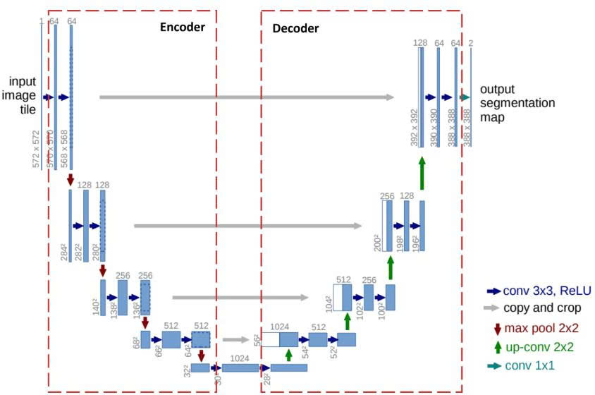
Figure 3: U-Net Architecture

The U-Net structure performs two main tasks:

1. Classification: Answering "What is this object?". To do this, U-Net compresses the image.

2. Localization: Identifying the coordinates of the object in the image space. To do this, U-Net needs to maintain the image size to avoid losing sharpness in boundaries.

U-Net resolves this conflict with its U-shape: the left side is responsible for "Compressing to Understand," while the right side is responsible for "Decompressing to Locate," with "bridges" connecting the two to merge this information.

2.1 Key Concepts in U-Net

2.1.1 Skip Connections

In encoder-decoder models, downsampling in the encoding branch often leads to significant data loss. To solve this, Skip Connections are used. Instead of forcing all information through the "bottleneck," skip connections establish a direct path from the encoder to the decoder.

Example: Think of it like a high-speed bypass. While the main road (the bottleneck) summarizes the general "idea" of the image, the skip connection carries the "original blueprint" (fine spatial details) directly to the construction site (the decoder) so it knows exactly where to place each pixel.

2.1.2 Convolution and Transposed Convolution

Convolution is the core of a CNN. It slides a filter (kernel) over the input to create feature maps. This process usually reduces the spatial dimensions.

Steps for Convolution:
- B1: Place the Kernel on the input.
- B2: Apply Padding (adding zeros) to keep the size or handle edges.
- B3: Element-wise multiplication.
- B4: Summation of the results.
- B5: Slide the kernel based on the Stride.

Concrete Example:

Input ($3 \times 3$):$$\begin{bmatrix} 1 & 2 & 3 \\ 4 & 5 & 6 \\ 7 & 8 & 9 \end{bmatrix}$$Kernel ($2 \times 2$):$$\begin{bmatrix} 1 & 0 \\ 0 & 1 \end{bmatrix}$$

Stride: 1, Padding: 0.

Step 1 (Top-left): $(1 \times 1) + (2 \times 0) + (4 \times 0) + (5 \times 1) = \mathbf{6}$

Step 2 (Top-right): $(2 \times 1) + (3 \times 0) + (5 \times 0) + (6 \times 1) = \mathbf{8}$

Final Output: $\begin{bmatrix} 6 & 8 \\ 12 & 14 \end{bmatrix}$ (Size reduced).

Transposed Convolution (Deconvolution) is used to increase the size of the data (upsampling).

Steps for Transposed Convolution:
- B1: Take an input pixel.
- B2: Multiply it by the entire Kernel.
- B3: Place the result into the output matrix.
- B4: Sum overlapping regions.

Concrete Example:

Input ($2 \times 2$): $\begin{bmatrix} a & b \\ c & d \end{bmatrix}$, Kernel ($2 \times 2$): $\begin{bmatrix} x & y \\ z & t \end{bmatrix}$

Stride = 1, Padding = 0.

Process pixel $a$: Result 1 = $\begin{bmatrix} ax & ay \\ az & at \end{bmatrix}$

Process pixel $b$: Result 2 = $\begin{bmatrix} bx & by \\ bz & bt \end{bmatrix}$ (shifted right).

Overlap: The column between $a$ and $b$ will be $ay + bx$.

In essence, while Convolution uses a kernel to aggregate pixels into a single feature, Transposed Convolution does the opposite: mapping a sparse feature into multiple pixels to expand the feature map (by adjusting padding and stride).

The superiority of Transposed Convolution over basic interpolation techniques (such as Nearest Neighbors, Bi-Linear Interpolation, or Max-Unpooling) lies in its ability to self-learn weights during training, allowing for a sharper and more accurate reconstruction of spatial details.

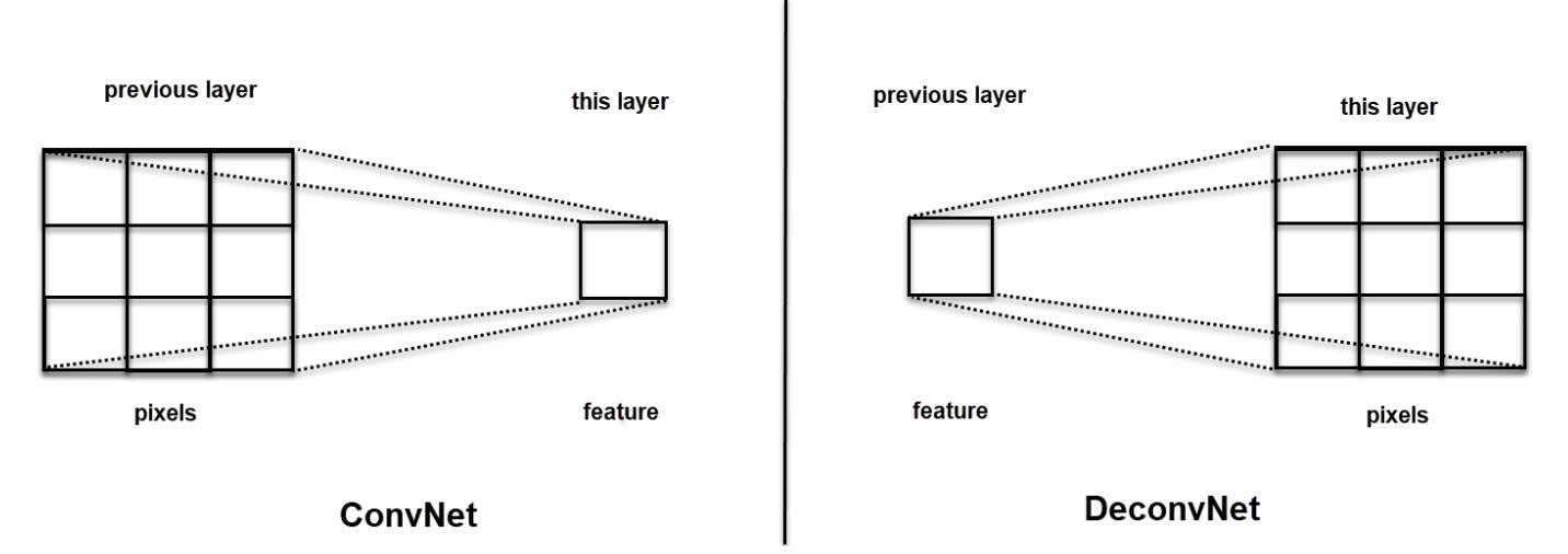
Figure 4: ConvNet vs DeconvNet

2.1.3 Max Pooling

A downsampling technique that slides a window over the feature map and keeps only the maximum value (the most prominent feature).

Example: In a $2 \times 2$ area with values $[1, 5, 2, 3]$, Max Pooling will only keep 5. This reduces data size by $75\%$ while keeping the most "important" signal.

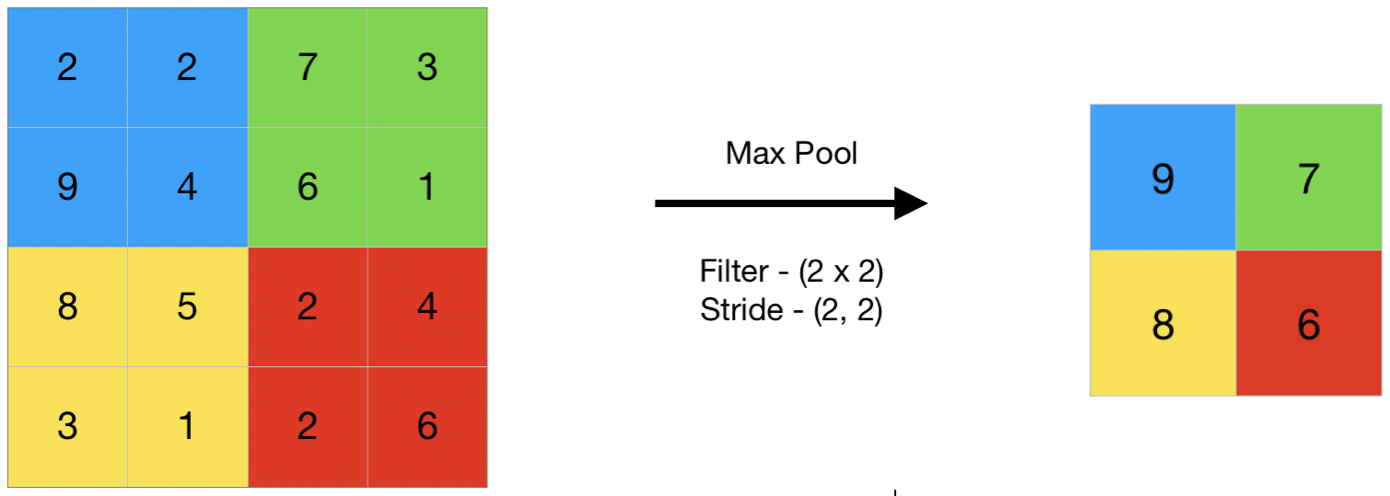
Figure 5: Max Pooling (Source: https://www.geeksforgeeks.org/deep-learning/cnn-introduction-to-pooling-layer/)

2.2 The Contracting Path (Encoder) - Left Side

The goal is Feature Extraction. The image goes down a series of "steps." As it goes deeper, the image size (width/height) decreases, but the depth (number of channels) increases.

Each step consists of:

1. Two $3 \times 3$ Convolutions + ReLU activation: Filters search for features (edges, corners).

2. $2 \times 2$ Max Pooling: Reduces dimensions by exactly half.

2.3 The Bottleneck

The bottom of the U where the image is most compressed. It contains two $3 \times 3$ Convolutions + ReLU. The number of channels reaches its peak here (usually 1024).

2.4 The Expanding Path (Decoder) - Right Side

U-Net now "climbs up" to restore the original image size.

Each step up consists of:

1. Transposed Convolution ($2 \times 2$): Doubles the dimensions and halves the channels.

2. Skip Connection (Concatenate): Data from the corresponding Encoder level is "pasted" onto the current layer to restore lost sharpness.

3. Two $3 \times 3$ Convolutions + ReLU: Smooths and blends the combined information.

2.5 Output Layer

After climbing back up, we use a $1 \times 1$ Convolution. This layer doesn't change the height or width; it simply collapses the many channels down to the exact number of classes you want to classify (e.g., if you are segmenting "cells" vs "background," the output channels will be 2).

2.6 Activation Functions

Activation functions enable the model to learn complex non-linear relationships within image data. In U-Net, their usage is generally categorized into two main groups:

2.6.1. Activation Functions for hidden layers (Encoder and Decoder Paths):

In every layer of the contracting (encoder) and expanding (decoder) paths—except for the final output—U-Net typically employs the ReLU (Rectified Linear Unit) activation function.

Characteristics:
- Formula: $f(x) = \max(0, x)$
- Mechanism: It passes all positive values through unchanged while mapping all negative values to zero.

Why it's used:

ReLU is the industry standard because it allows the model to train much faster and effectively solves the "Vanishing Gradient" problem that plagued older functions like Sigmoid or Tanh in deep networks.

2.6.2 Activation Functions for the Output Layer

This is the most critical part because it determines the format of your prediction. The choice depends entirely on the type of segmentation task you are solving.

2.6.2.1 Sigmoid (For Binary Segmentation)

Used when you only have two classes: "Object" and "Background."

Formula:$$\sigma(x) = \frac{1}{1 + e^{-x}}$$

Output Range: $[0, 1]$ (interpreted as a probability).

2.6.2.2 Softmax (For Multi-class Segmentation)

Used when you need to distinguish between three or more different categories.

Formula:$$\text{Softmax}(x_i) = \frac{e^{x_i}}{\sum e^{x_j}}$$

3. Hands-on Image Segmentation with U-Net in PyTorch

3.1. Import Libraries

First, we need to import the necessary libraries for data processing and model building.

%matplotlib inline

import numpy as np
import random
import time
import copy
from collections import defaultdict
from functools import reduce

import matplotlib.pyplot as plt

import torch
import torch.nn as nn
import torch.nn.functional as F
import torch.optim as optim
from torch.optim import lr_scheduler
from torch.utils.data import Dataset, DataLoader
from torchvision import transforms

device = torch.device('cuda' if torch.cuda.is_available() else 'cpu')
print(f'Using device: {device}')

3.2. Create Synthetic Data

To make it easier to practice, we will generate our own image dataset. Each image will contain 6 different shapes, including:
1. Filled square
2. Filled circle
3. Triangle
4. Circle outline
5. Mesh square
6. Plus sign

The model's goal is to take an input image (containing all shapes overlaid on each other), and produce 6 separate masks, each identifying the location of one type of shape.

Below are the functions to generate the data:

# ============================================================
# Basic shape drawing functions
# ============================================================

def logical_and(arrays):
    """Perform logical AND on multiple arrays at once."""
    new_array = np.ones(arrays[0].shape, dtype=bool)
    for a in arrays:
        new_array = np.logical_and(new_array, a)
    return new_array

def add_filled_square(arr, x, y, size):
    """Draw a filled square at position (x, y)."""
    s = int(size / 2)
    xx, yy = np.mgrid[:arr.shape[0], :arr.shape[1]]
    return np.logical_or(arr, logical_and([xx > x - s, xx < x + s, yy > y - s, yy < y + s]))

def add_mesh_square(arr, x, y, size):
    """Draw a mesh square at position (x, y)."""
    s = int(size / 2)
    xx, yy = np.mgrid[:arr.shape[0], :arr.shape[1]]
    return np.logical_or(arr, logical_and([xx > x - s, xx < x + s, xx % 2 == 1, yy > y - s, yy < y + s, yy % 2 == 1]))

def add_triangle(arr, x, y, size):
    """Draw a triangle at position (x, y)."""
    s = int(size / 2)
    triangle = np.tril(np.ones((size, size), dtype=bool))
    arr[x-s:x-s+triangle.shape[0], y-s:y-s+triangle.shape[1]] = triangle
    return arr

def add_circle(arr, x, y, size, fill=False):
    """Draw a circle (filled or outline) at position (x, y)."""
    xx, yy = np.mgrid[:arr.shape[0], :arr.shape[1]]
    circle = np.sqrt((xx - x) ** 2 + (yy - y) ** 2)
    new_arr = np.logical_or(arr, np.logical_and(circle < size, circle >= size * 0.7 if not fill else True))
    return new_arr

def add_plus(arr, x, y, size):
    """Draw a plus sign (+) at position (x, y)."""
    s = int(size / 2)
    arr[x-1:x+1, y-s:y+s] = True
    arr[x-s:x+s, y-1:y+1] = True
    return arr

def get_random_location(width, height, zoom=1.0):
    """Generate a random location within the frame."""
    x = int(width * random.uniform(0.1, 0.9))
    y = int(height * random.uniform(0.1, 0.9))
    size = int(min(width, height) * random.uniform(0.06, 0.12) * zoom)
    return (x, y, size)

# ============================================================
# Image and mask generation functions
# ============================================================

def generate_img_and_mask(height, width):
    """
    Generate ONE image and 6 corresponding masks.

    Returns:
        arr: Input image (1, H, W) - all shapes overlaid
        masks: 6 separate masks (6, H, W) - one mask per shape type
    """
    shape = (height, width)

    # Generate random position for each shape
    triangle_location = get_random_location(*shape)
    circle_location1 = get_random_location(*shape, zoom=0.7)
    circle_location2 = get_random_location(*shape, zoom=0.5)
    mesh_location = get_random_location(*shape)
    square_location = get_random_location(*shape, zoom=0.8)
    plus_location = get_random_location(*shape, zoom=1.2)

    # Create input image: draw ALL shapes on the same image
    arr = np.zeros(shape, dtype=bool)
    arr = add_triangle(arr, *triangle_location)
    arr = add_circle(arr, *circle_location1)
    arr = add_circle(arr, *circle_location2, fill=True)
    arr = add_mesh_square(arr, *mesh_location)
    arr = add_filled_square(arr, *square_location)
    arr = add_plus(arr, *plus_location)
    arr = np.reshape(arr, (1, height, width)).astype(np.float32)

    # Create target masks: each shape has its OWN mask
    masks = np.asarray([
        add_filled_square(np.zeros(shape, dtype=bool), *square_location),     # Mask 0: Filled square
        add_circle(np.zeros(shape, dtype=bool), *circle_location2, fill=True),# Mask 1: Filled circle
        add_triangle(np.zeros(shape, dtype=bool), *triangle_location),        # Mask 2: Triangle
        add_circle(np.zeros(shape, dtype=bool), *circle_location1),           # Mask 3: Circle outline
        add_filled_square(np.zeros(shape, dtype=bool), *mesh_location),       # Mask 4: Mesh square
        add_plus(np.zeros(shape, dtype=bool), *plus_location)                 # Mask 5: Plus sign
    ]).astype(np.float32)

    return arr, masks

def generate_random_data(height, width, count):
    """
    Generate `count` random images with corresponding masks.

    Returns:
        X: Input images (count, H, W, 3) - RGB
        Y: Target masks (count, 6, H, W)
    """
    x, y = zip(*[generate_img_and_mask(height, width) for i in range(0, count)])

    X = np.asarray(x) * 255
    X = X.repeat(3, axis=1).transpose([0, 2, 3, 1]).astype(np.uint8)
    Y = np.asarray(y)

    return X, Y

# ============================================================
# Visualization functions
# ============================================================

def plot_img_array(img_array, ncol=3):
    """Display an array of images as a grid."""
    nrow = len(img_array) // ncol
    _, plots = plt.subplots(nrow, ncol, sharex='all', sharey='all', figsize=(ncol * 4, nrow * 4))
    for i in range(len(img_array)):
        plots[i // ncol, i % ncol].imshow(img_array[i])
    plt.tight_layout()

def plot_side_by_side(img_arrays):
    """Display multiple groups of images side by side for comparison."""
    flatten_list = reduce(lambda x, y: x + y, zip(*img_arrays))
    plot_img_array(np.array(flatten_list), ncol=len(img_arrays))

def masks_to_colorimg(masks):
    """
    Convert 6 masks (each a single channel) into an RGB color image.
    Each shape type is assigned a different color.
    """
    colors = np.asarray([
        (201, 58, 64),    # Red        - Filled square
        (242, 207, 1),    # Yellow     - Filled circle
        (0, 152, 75),     # Green      - Triangle
        (101, 172, 228),  # Blue       - Circle outline
        (56, 34, 132),    # Purple     - Mesh square
        (160, 194, 56)    # Lime green - Plus sign
    ])

    colorimg = np.ones((masks.shape[1], masks.shape[2], 3), dtype=np.float32) * 255
    channels, height, width = masks.shape

    for y in range(height):
        for x in range(width):
            selected_colors = colors[masks[:, y, x] > 0.5]
            if len(selected_colors) > 0:
                colorimg[y, x, :] = np.mean(selected_colors, axis=0)

    return colorimg.astype(np.uint8)

3.3. Visualize Synthetic Data

After defining the drawing functions, let's generate some sample data to better understand the model's objective. Below are 3 examples along with their corresponding masks. The image pairs are displayed row by row:
- Left column (Input image): You can see all shapes drawn on top of each other on a black background. This is what the model will "see."
- Right column (Target mask): Each shape is colored differently. This is the "answer" that the model needs to learn to predict.

We will build a U-Net model to take images from the left column and predict masks as close to the right column as possible.

# Generate 3 sample images
input_images, target_masks = generate_random_data(192, 192, count=3)

# Convert masks to color images for visualization
input_images_rgb = [x.astype(np.uint8) for x in input_images]
target_masks_rgb = [masks_to_colorimg(x) for x in target_masks]

# Display: Left = Input image, Right = Target mask
plot_side_by_side([input_images_rgb, target_masks_rgb])

Figure 6: Input images (left) and corresponding target masks (right) — each color represents a different shape type to segment.

View each individual mask in detail

To gain a better understanding, let's look at the 6 separate masks for one image:

# View each individual mask of the first image
mask_names = ['Filled Square', 'Filled Circle', 'Triangle', 'Circle Outline', 'Mesh Square', 'Plus Sign']

fig, axes = plt.subplots(2, 4, figsize=(16, 8))

# Original image
axes[0, 0].imshow(input_images[0])
axes[0, 0].set_title('Input Image', fontsize=12)

# Composite mask
axes[0, 1].imshow(target_masks_rgb[0])
axes[0, 1].set_title('Composite Mask (colored)', fontsize=12)

# Hide 2 empty cells
axes[0, 2].axis('off')
axes[0, 3].axis('off')

# 6 individual masks
colors_map = ['Reds', 'YlOrBr', 'Greens', 'Blues', 'Purples', 'YlGn']
for i in range(6):
    row = (i + 2) // 4
    col = (i + 2) % 4
    axes[row, col].imshow(target_masks[0][i], cmap=colors_map[i])
    axes[row, col].set_title(f'Mask {i}: {mask_names[i]}', fontsize=11)

plt.tight_layout()
plt.show()

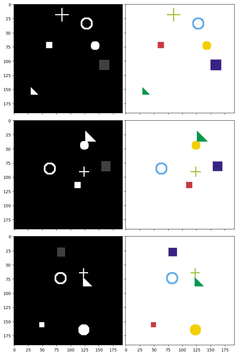
Figure 7: Input image and 6 corresponding ground truth masks — each mask contains only one type of shape to segment.

3.4. Create Dataset and DataLoader

PyTorch uses two important concepts:

• Dataset: Where data is stored, providing a way to access each sample
• DataLoader: Automatically splits data into batches, shuffles, etc.

We will create:
- 2000 images for the training set
- 200 images for the validation set

class SimDataset(Dataset):
    """
    Dataset containing randomly generated shape images.
    Inherits from torch.utils.data.Dataset.
    """
    def __init__(self, count, transform=None):
        # Generate all images at dataset initialization
        self.input_images, self.target_masks = generate_random_data(192, 192, count=count)
        self.transform = transform

    def __len__(self):
        return len(self.input_images)

    def __getitem__(self, idx):
        image = self.input_images[idx]
        mask = self.target_masks[idx]
        if self.transform:
            image = self.transform(image)
        return [image, mask]

# Transform: convert numpy array → PyTorch Tensor
trans = transforms.Compose([
    transforms.ToTensor(),  # Convert (H, W, C) → (C, H, W) and scale [0, 255] → [0, 1]
])

# Create datasets
train_set = SimDataset(2000, transform=trans)
val_set = SimDataset(200, transform=trans)

# Create DataLoaders
batch_size = 25

dataloaders = {
    'train': DataLoader(train_set, batch_size=batch_size, shuffle=True, num_workers=0),
    'val': DataLoader(val_set, batch_size=batch_size, shuffle=True, num_workers=0)
}

dataset_sizes = {x: len(ds) for x, ds in zip(['train', 'val'], [train_set, val_set])}

# Check a data batch
def reverse_transform(inp):
    """Convert tensor (C, H, W) back to numpy RGB (H, W, C) for display."""
    inp = inp.numpy().transpose((1, 2, 0))
    inp = np.clip(inp, 0, 1)
    inp = (inp * 255).astype(np.uint8)
    return inp

inputs, masks = next(iter(dataloaders['train']))
print(f'Batch inputs shape: {inputs.shape}')  # (25, 3, 192, 192)
print(f'Batch masks shape:  {masks.shape}')    # (25, 6, 192, 192)

# Display one image from the batch
plt.figure(figsize=(5, 5))
plt.imshow(reverse_transform(inputs[0]))
plt.title('A sample image from the training batch')
plt.axis('off')
plt.show()

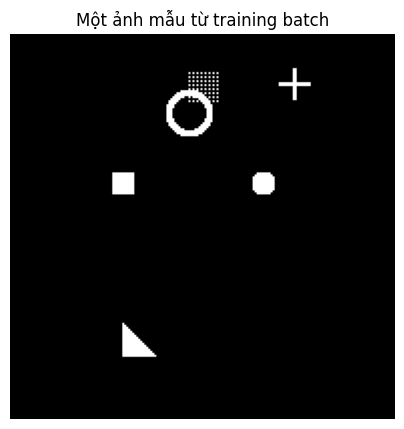
Figure 8: The input the model receives: 6 randomly drawn shapes overlaid on a black background.

3.5. Build the U-Net Model

Double Convolution Block

This is the fundamental "building block" of U-Net. Every level in U-Net uses 2 consecutive Convolution layers:

Input → Conv2d(3×3) → ReLU → Conv2d(3×3) → ReLU → Output

• Conv2d(3×3): Convolution layer with a 3×3 kernel, padding=1 to preserve spatial dimensions
• ReLU: Activation function, enabling the network to learn non-linear relationships

We use 2 consecutive Conv layers to help the network extract richer features at each level.

def double_conv(in_channels, out_channels):
    """
    Double Convolution block: Conv → ReLU → Conv → ReLU
    Preserves spatial dimensions (H, W) thanks to padding=1.
    """
    return nn.Sequential(
        nn.Conv2d(in_channels, out_channels, kernel_size=3, padding=1),
        nn.ReLU(inplace=True),
        nn.Conv2d(out_channels, out_channels, kernel_size=3, padding=1),
        nn.ReLU(inplace=True)
    )

Complete U-Net Model

Below is the U-Net model with the following architecture:

Figure 9: U-Net Architecture [2]

Note: In the Decoder, when we concatenate feature maps from the Encoder via skip connections, the number of channels adds up. For example: 512 (from Bottleneck) + 256 (from skip) = 768 input channels for dconv_up3.

class UNet(nn.Module):
    """
    U-Net model for Image Segmentation.

    Args:
        n_class: Number of classes to segment (= number of output masks)
    """

    def __init__(self, n_class):
        super().__init__()

        # === ENCODER (downward path) ===
        self.dconv_down1 = double_conv(3, 64)       # (3, H, W) → (64, H, W)
        self.dconv_down2 = double_conv(64, 128)     # (64, H/2, W/2) → (128, H/2, W/2)
        self.dconv_down3 = double_conv(128, 256)    # (128, H/4, W/4) → (256, H/4, W/4)
        self.dconv_down4 = double_conv(256, 512)    # (256, H/8, W/8) → (512, H/8, W/8)  ← Bottleneck

        # MaxPool halves the spatial dimensions
        self.maxpool = nn.MaxPool2d(2)
        # Upsample doubles the spatial dimensions
        self.upsample = nn.Upsample(scale_factor=2, mode='bilinear', align_corners=True)

        # === DECODER (upward path) ===
        # Note: input channels = upsampled channels + skip channels
        self.dconv_up3 = double_conv(256 + 512, 256)  # (768, H/4, W/4) → (256, H/4, W/4)
        self.dconv_up2 = double_conv(128 + 256, 128)  # (384, H/2, W/2) → (128, H/2, W/2)
        self.dconv_up1 = double_conv(128 + 64, 64)    # (192, H, W)     → (64, H, W)

        # Final layer: convert 64 channels → n_class channels (each channel = 1 mask)
        self.conv_last = nn.Conv2d(64, n_class, kernel_size=1)

    def forward(self, x):
        # ========== ENCODER ==========
        conv1 = self.dconv_down1(x)         # Save for skip connection
        x = self.maxpool(conv1)             # Downsample ×2

        conv2 = self.dconv_down2(x)         # Save for skip connection
        x = self.maxpool(conv2)             # Downsample ×2

        conv3 = self.dconv_down3(x)         # Save for skip connection
        x = self.maxpool(conv3)             # Downsample ×2

        # ========== BOTTLENECK ==========
        x = self.dconv_down4(x)             # Most compressed representation

        # ========== DECODER ==========
        x = self.upsample(x)                # Upsample ×2
        x = torch.cat([x, conv3], dim=1)    # Concatenate with skip connection from encoder
        x = self.dconv_up3(x)

        x = self.upsample(x)                # Upsample ×2
        x = torch.cat([x, conv2], dim=1)    # Concatenate with skip connection
        x = self.dconv_up2(x)

        x = self.upsample(x)                # Upsample ×2
        x = torch.cat([x, conv1], dim=1)    # Concatenate with skip connection
        x = self.dconv_up1(x)

        # Final layer: convert to n_class channels
        out = self.conv_last(x)

        return out

3.6. Loss Function

To train the model, we need a loss function to measure how far the model's predictions are from the ground truth. We will combine 2 popular loss functions for segmentation tasks:

3.6.1. Binary Cross-Entropy (BCE)

This loss function performs binary classification for each pixel, helping the model accurately determine whether each pixel belongs to a given shape region or not.

3.6.2. Dice Loss

Dice Loss is an important loss function used to measure the overlap between the predicted region and the ground truth in image segmentation tasks. Dice Loss values range from 0 to 1, corresponding to states from perfect overlap to no overlap at all. Its key advantage is the ability to effectively handle class imbalance, which is particularly useful when the target object occupies a very small area relative to the entire image.

Mathematically, the Dice Loss formula is defined as follows:
$$\text{Dice} = 1 - \frac{2 \times |A \cap B|}{|A| + |B|}$$

Where $A$ represents the model's predicted region, $B$ is the ground truth region, and $|A \cap B|$ denotes the intersection between the two regions.

3.6.3. Combined BCE + Dice

We combine the two loss functions into the main loss function:
$$\text{Loss} = 0.5 \times \text{BCE} + 0.5 \times \text{Dice}$$

This combination helps the model correctly classify each pixel (BCE) while also ensuring the overall shape accuracy (Dice).

def dice_loss(pred, target, smooth=1.):
    """
    Compute Dice Loss between prediction and target.

    Args:
        pred: Model prediction (after sigmoid), shape (N, C, H, W)
        target: Ground truth mask, shape (N, C, H, W)
        smooth: Smoothing factor to avoid division by zero
    """
    pred = pred.contiguous()
    target = target.contiguous()

    # Compute intersection
    intersection = (pred * target).sum(dim=2).sum(dim=2)

    # Compute Dice coefficient then convert to loss
    loss = (1 - ((2. * intersection + smooth) /
                 (pred.sum(dim=2).sum(dim=2) + target.sum(dim=2).sum(dim=2) + smooth)))

    return loss.mean()


def calc_loss(pred, target, metrics, bce_weight=0.5):
    """
    Compute total loss = BCE + Dice.
    Also record metrics for monitoring.
    """
    bce = F.binary_cross_entropy_with_logits(pred, target)

    pred = torch.sigmoid(pred)  # Convert logits → probabilities [0, 1]
    dice = dice_loss(pred, target)

    loss = bce * bce_weight + dice * (1 - bce_weight)

    metrics['bce'] += bce.data.cpu().numpy() * target.size(0)
    metrics['dice'] += dice.data.cpu().numpy() * target.size(0)
    metrics['loss'] += loss.data.cpu().numpy() * target.size(0)

    return loss

3.7. Train the Model

3.7.1. Training Loop

This is the "engine" of the training process. Each epoch consists of 2 phases:

1. Training phase: The model learns from data and updates weights
2. Validation phase: The model is evaluated on unseen data, with no weight updates

We also save the best model (the one with the lowest validation loss) for later use.

def print_metrics(metrics, epoch_samples, phase):
    """Print metrics for a given phase."""
    outputs = []
    for k in metrics.keys():
        outputs.append("{}: {:.4f}".format(k, metrics[k] / epoch_samples))
    print("{}: {}".format(phase, ", ".join(outputs)))


def train_model(model, optimizer, scheduler, num_epochs=25):
    """
    Main training loop.

    Args:
        model: U-Net model
        optimizer: Optimization algorithm (Adam)
        scheduler: Learning rate scheduler
        num_epochs: Number of training epochs

    Returns:
        model: Model with the best weights
    """
    best_model_wts = copy.deepcopy(model.state_dict())
    best_loss = 1e10

    # Store loss history for plotting
    history = {'train_loss': [], 'val_loss': []}

    for epoch in range(num_epochs):
        print(f'Epoch {epoch}/{num_epochs - 1}')
        print('-' * 30)

        since = time.time()

        # Each epoch has 2 phases: train and val
        for phase in ['train', 'val']:
            if phase == 'train':
                model.train()   # Enable training mode (dropout, batchnorm active)
            else:
                model.eval()    # Enable evaluation mode

            metrics = defaultdict(float)
            epoch_samples = 0

            for inputs, labels in dataloaders[phase]:
                inputs = inputs.to(device)
                labels = labels.to(device)

                # Clear old gradients
                optimizer.zero_grad()

                # Forward pass
                with torch.set_grad_enabled(phase == 'train'):
                    outputs = model(inputs)
                    loss = calc_loss(outputs, labels, metrics)

                    # Backward + update only during training
                    if phase == 'train':
                        loss.backward()
                        optimizer.step()

                epoch_samples += inputs.size(0)

            print_metrics(metrics, epoch_samples, phase)
            epoch_loss = metrics['loss'] / epoch_samples

            # Record loss
            if phase == 'train':
                history['train_loss'].append(epoch_loss)
            else:
                history['val_loss'].append(epoch_loss)

            # Save the best model
            if phase == 'val' and epoch_loss < best_loss:
                print("  → Saving best model!")
                best_loss = epoch_loss
                best_model_wts = copy.deepcopy(model.state_dict())

        # Update learning rate
        scheduler.step()

        time_elapsed = time.time() - since
        print(f'Time: {time_elapsed // 60:.0f}m {time_elapsed % 60:.0f}s\n')

    print(f'\nBest val loss: {best_loss:.4f}')

    # Load the best weights
    model.load_state_dict(best_model_wts)
    return model, history

3.7.2. Train the Model

We will use:
- Adam optimizer: A popular optimization algorithm that automatically adjusts the learning rate for each parameter
- Learning rate = 1e-4: Initial learning rate
- StepLR scheduler: Reduces the learning rate by a factor of 10 every 25 epochs
- 40 epochs: Number of passes through the entire dataset

num_class = 6  # Number of masks to predict

# Initialize the model (ensure starting from scratch)
model = UNet(num_class).to(device)

# Optimizer: Adam with learning rate = 0.0001
optimizer = optim.Adam(model.parameters(), lr=1e-4)

# Scheduler: reduce LR ×0.1 every 25 epochs
scheduler = lr_scheduler.StepLR(optimizer, step_size=25, gamma=0.1)

# Start training
model, history = train_model(model, optimizer, scheduler, num_epochs=40)

Loss Over Epochs

After training is complete, let's see how the loss decreases during training:

# Plot training/validation loss
plt.figure(figsize=(10, 5))
plt.plot(history['train_loss'], label='Train Loss', linewidth=2)
plt.plot(history['val_loss'], label='Validation Loss', linewidth=2)
plt.xlabel('Epoch', fontsize=12)
plt.ylabel('Loss', fontsize=12)
plt.title('Training & Validation Loss Over Epochs', fontsize=14)
plt.legend(fontsize=12)
plt.grid(True, alpha=0.3)
plt.tight_layout()
plt.show()

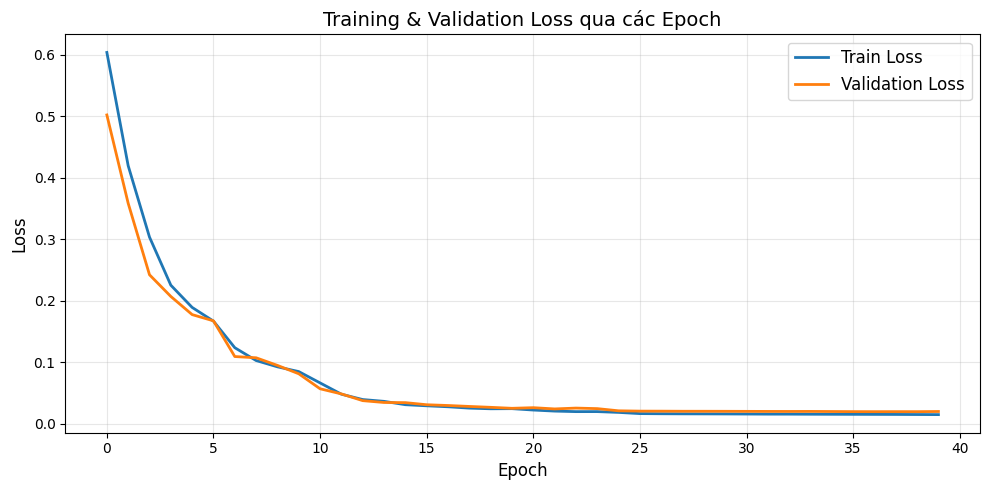
Figure 10: Training process

We can see that the loss drops rapidly in the first 10 epochs (from 0.6 down to 0.05), indicating the model learns the main data features very early. After epoch 15, both curves nearly flatten and converge to a very low value (~0.02), proving the model has learned well and stabilized. We also observe that the training loss and validation loss closely track each other throughout training, showing that the model is not overfitting.

3.8. Evaluate Results — What Has the Model Learned?

We will generate new data (that the model has never seen) and examine how the model predicts. To evaluate the model's results and compare, we will display 3 columns:
1. Input image: What the model "sees"
2. Ground Truth mask: The correct answer
3. Model Prediction: The result the model produces

# Switch model to evaluation mode
model.eval()

# Generate NEW test data (the model has never seen this)
test_dataset = SimDataset(3, transform=trans)
test_loader = DataLoader(test_dataset, batch_size=3, shuffle=False, num_workers=0)

# Get a batch
inputs, labels = next(iter(test_loader))
inputs = inputs.to(device)
labels = labels.to(device)

# Predict (no gradient computation needed)
with torch.no_grad():
    pred = model(inputs)

pred = pred.data.cpu().numpy()
print(f'Output shape: {pred.shape}')  # (3, 6, 192, 192)

# Prepare images for display
input_images_rgb = [reverse_transform(x) for x in inputs.cpu()]
target_masks_rgb = [masks_to_colorimg(x) for x in labels.cpu().numpy()]
pred_rgb = [masks_to_colorimg(x) for x in pred]

# Display results
print('Left → Right: Input Image | Ground Truth Mask | Model Prediction')
print('=' * 60)
plot_side_by_side([input_images_rgb, target_masks_rgb, pred_rgb])

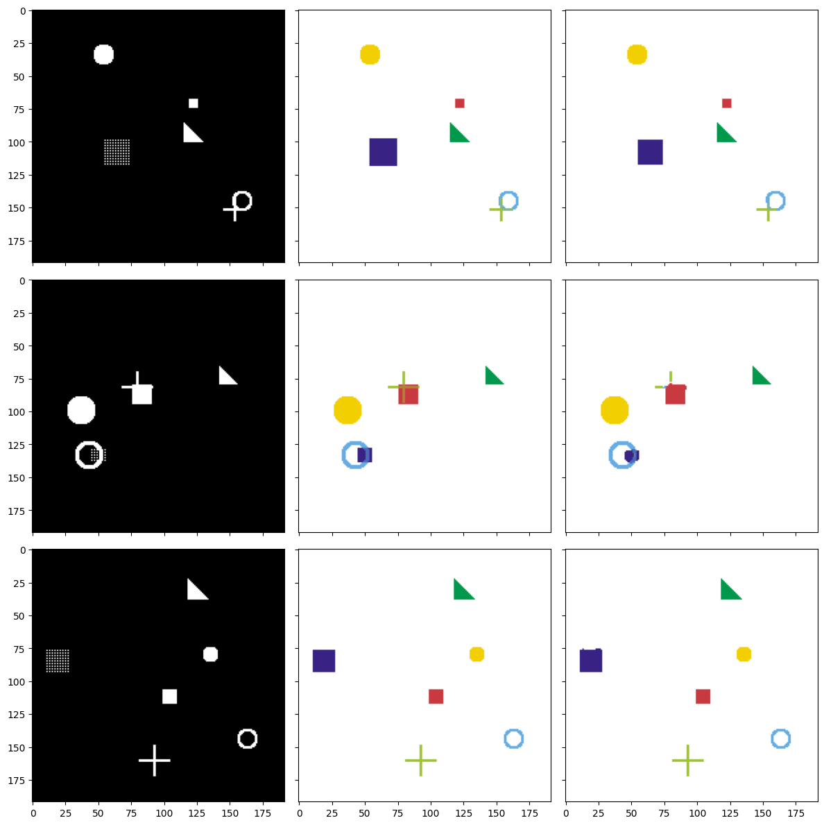
Figure 11: Three test samples: input image (left) — ground truth mask (center) — model prediction (right).

Result Analysis

Looking at the figure, we can see that the Prediction column (right) closely matches the Ground Truth column (center). This demonstrates that the model has learned to distinguish different shapes, correctly identify the position of each object in the image, and produce a separate mask for each shape type.

Predictions may not be 100% perfect, especially at the edges — this is completely normal. In practice, results can be improved by adding more training data, increasing the number of epochs, applying techniques such as Batch Normalization, Dropout, or using Data Augmentation.

Detailed View of Each Predicted Mask

Let's compare each mask in detail:

# Detailed comparison of each mask for the first image
mask_names = ['Filled Square', 'Filled Circle', 'Triangle', 'Circle Outline', 'Mesh Square', 'Plus Sign']

fig, axes = plt.subplots(6, 3, figsize=(12, 24))
fig.suptitle('Detailed Comparison of Each Mask (Image #1)', fontsize=16, y=1.01)

for i in range(6):
    # Column 1: Original image
    axes[i, 0].imshow(input_images_rgb[0])
    axes[i, 0].set_title(f'Input Image' if i == 0 else '')
    axes[i, 0].set_ylabel(mask_names[i], fontsize=12, rotation=0, labelpad=80)

    # Column 2: Ground truth mask
    axes[i, 1].imshow(labels.cpu().numpy()[0][i], cmap='gray')
    axes[i, 1].set_title('Ground Truth' if i == 0 else '')

    # Column 3: Predicted mask (apply sigmoid to convert to [0, 1])
    pred_sigmoid = 1 / (1 + np.exp(-pred[0][i]))  # sigmoid
    axes[i, 2].imshow(pred_sigmoid, cmap='gray')
    axes[i, 2].set_title('Prediction' if i == 0 else '')

for ax in axes.flat:
    ax.set_xticks([])
    ax.set_yticks([])

plt.tight_layout()
plt.show()

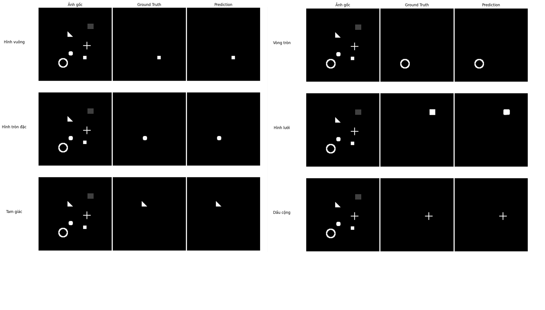
Figure 12: Ground Truth vs. Prediction comparison for each individual mask.

Looking at each Ground Truth - Prediction pair, we can see that the model predicts the position and shape of all 6 classes very accurately. In particular, shapes with clear outlines like the circle outline, triangle, and plus sign are reproduced almost perfectly. For the mesh square, the model predicts a solid square instead of a dotted grid — this makes sense because the mesh square's ground truth mask is also represented as a filled square during data generation. Overall, the results show that U-Net has learned this segmentation task well after just 40 training epochs.

3.9. Future Directions

If you want to explore further, try:

1. Modify the architecture: Add Batch Normalization, Dropout, or use ResNet as the Encoder
2. Use real-world data: Try datasets like COCO, Pascal VOC, or medical images
3. Data Augmentation: Rotation, flipping, color changes... to help the model generalize better
4. U-Net variants: U-Net++, Attention U-Net, V-Net (3D)

References

[1] N. Usuyama, "pytorch-unet," GitHub, [Online]. Available: https://github.com/usuyama/pytorch-unet. [Accessed: 15-Mar-2026]

[2] O. Ronneberger, P. Fischer, and T. Brox, "U-Net: Convolutional Networks for Biomedical Image Segmentation," arXiv:1505.04597, May 2015. [Online]. Available: https://arxiv.org/pdf/1505.04597. [Accessed: 15-Mar-2026]