
Introduction
In this blog, we will build a complete Machine Learning project "Predicting Student Test Scores" from Data Analysis to Model Deployment using Gradio. Student test score prediction will be based on features in the data such as study_hours, study_method, sleep_hours, class_attendance,... This is a typical regression problem, very suitable for those who are new to ML or want a practical project to add to their portfolio.
1. Problem Definition & Scope Identification
Objective: Build a model to predict student test scores based on input factors such as study hours, study habits, sleep quality...
1.1. Problem Identification
This is a Regression Problem - a type of supervised learning problem in Machine Learning.
What is Regression?
- Regression is a problem that predicts a continuous value instead of classifying into discrete groups
- Examples: Predicting house prices (1.5 billion, 2.3 billion...), temperature (25.5°C, 30.2°C...), or in this case test scores (75.5, 82.3, 90.0...)
- Different from Classification which only predicts discrete labels (such as "Pass/Fail")
Identifying the Target Variable:
- In this dataset, we will predict the variable: exam_score
- This is a continuous variable with values from 0-100 points
1.2. Evaluation Metrics
For regression problems, we DO NOT use Accuracy (Accuracy is only used for classification). Instead, we use the following metrics:
1. RMSE (Root Mean Squared Error):
RMSE = √(Σ(y_actual - y_predicted)²/n)
- Measures the average error between predicted and actual values
- Has the same unit as the target variable (points)
- Lower is better - RMSE = 8 means average error of ±8 points
- Sensitive to outliers (penalizes large errors more)
2. MAE (Mean Absolute Error):
MAE = Σ|y_actual - y_predicted|/n
- Average error regardless of positive/negative direction
- Easier to understand than RMSE
- Lower is better - MAE = 3 means average deviation of 3 points
- Less affected by outliers than RMSE
3. R² Score (Coefficient of Determination):
R² = 1 - (SS_residual / SS_total)
- Measures how much % of data variation the model explains
- Values from 0 to 1 (or negative if model is very poor)
- R² = 0.85 means the model explains 85% of variance in data
- Closer to 1 is better
4. MAPE (Mean Absolute Percentage Error) - optional:
MAPE = (100/n) × Σ|(y_actual - y_predicted)/y_actual|
- Error calculated as percentage
- Easy to understand for business: "Average deviation of 5%"
1.3. Questions to Answer:
- Which factors most influence test results?
- How accurate can the model predict (what RMSE, R²)?
- Are there hidden patterns in the data (non-linear correlations, interaction effects)?
- Is the model overfitting or underfitting?
- Can the results be trusted for real-world application?
2. Data Collection
In this project, we use data from Kaggle:
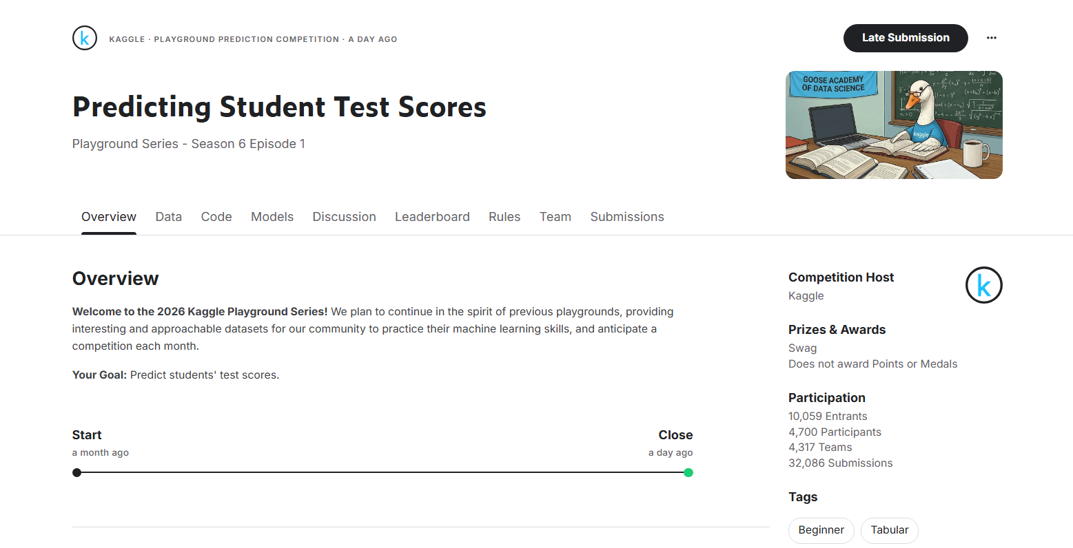
Dataset "Predicting Student Test Scores":
- Link: https://www.kaggle.com/competitions/playground-series-s6e1
We will use the dataset from Kaggle Tabular Playground Series Season 6 Episode 1 - a competition for ML learners with a short duration (a few weeks). The data is synthetically-generated from a deep learning model, providing a safe 'sandbox' environment for practice without worrying about leaking real information.
3. Exploratory Data Analysis (EDA)
EDA is an extremely important step in the ML process - this is where you truly "get to know" your data. A good EDA helps you:
- Deeply understand data characteristics through distribution and characteristics of each variable
- Detect problems in data (missing, duplicates, outliers, logic errors...)
- Discover relationships between variables and target
- Make correct decisions for subsequent steps
3.1. Load and Initial Data Exploration
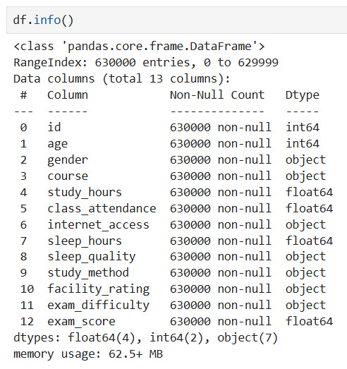
Observation: The data is very clean, with all 630,000 records containing complete information in all columns. This eliminates the complex preprocessing step of handling missing data.
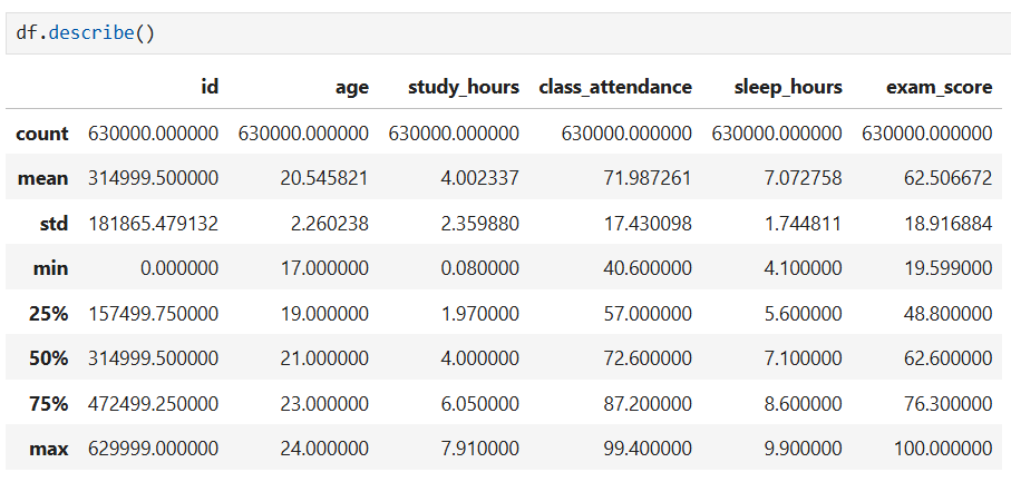
Observations:
- Large data scale: The very large dataset with 630,000 records shows high statistical reliability.
- Wide test score distribution: Average test score is 62.5 points, but with very large dispersion from 19.6 to 100 points, showing significant differences in academic performance among students.
- Average study time: Students spend an average of about 4 hours studying and sleep about 7 hours per day.
3.2. Finding Data Problems
This is the MOST IMPORTANT step to detect issues that need addressing.
3.2.1. Check for Missing Data
Purpose: Detect missing data - which columns are missing and by what percentage?
missing = df.isnull().sum()
If there is missing data:
- Missing < 5%: Can drop rows or impute
- Missing 5-30%: Should impute (mean, median, mode, KNN...)
- Missing > 30%: Consider dropping column or creating "missing indicator"
3.2.2. Check for Duplicate Rows
Purpose: Find duplicate rows - can cause overfitting or data leakage
duplicates = df.duplicated().sum()
3.2.3. Check for Outliers
Purpose: Detect abnormal values - could be errors or important insights
# IQR method
outlier_summary = []
for col in numeric_cols:
    Q1 = df[col].quantile(0.25)
    Q3 = df[col].quantile(0.75)
    IQR = Q3 - Q1
    lower = Q1 - 1.5 * IQR
    upper = Q3 + 1.5 * IQR

    outliers = df[(df[col] < lower) | (df[col] > upper)]
    outlier_summary.append({
        'Column': col,
        'Outliers_Count': len(outliers),
        'Percentage': len(outliers)/len(df)*100
    })

outlier_df = pd.DataFrame(outlier_summary).sort_values('Outliers_Count', ascending=False)
print(outlier_df)
IMPORTANT Note: Not all outliers should be removed!
- Outliers could be excellent/poor students
- Could be important patterns to keep
- Only remove if certain it's a data entry error
3.2.4. Check Data Format and Logic
Purpose: Check if data types are correct? Are there numbers mixed with text? Are dates in correct format?
- Check data types: Review and prevent inconsistencies between characters (strings) and numbers (numeric values), ensuring consistency for calculations.
- Validate formats: Verify structured information fields such as Dates, Emails, and Phone numbers according to system standards.
- Business logic: Apply customized validation algorithms according to the specificity of each variable, ensuring data is not only structurally correct but also fits the real context (example: Test scores must be 0-100, Study hours cannot be negative,...)
Observation:
This synthetic dataset "Predicting Student Test Scores" is basically clean, with no missing values, outliers, or logic errors => helping reduce the Data Cleaning workload!
3.3. Data Cleaning
Purpose: Address the issues identified in step 3.2
In other cases, data cleaning may include the following steps:
Summary table: Issues detected in EDA and How to handle them
| Issue Detected | How to Check | Evaluation Criteria | How to Handle | Notes |
|---|---|---|---|---|
| Missing Data | df.isnull().sum() |
- Missing < 5% - Missing 5-30% - Missing > 30% |
- < 5%: Drop rows or simple imputation (mean/median/mode) - 5-30%: Advanced imputation (KNN, Iterative) - > 30%: Drop column or create missing indicator |
Consider significance of missing data (random or pattern) |
| Duplicate Data | df.duplicated().sum() |
Number and % of duplicates | - Remove: df.drop_duplicates()- Keep first/last: keep='first'- Verify before removing |
May be valid duplicates (e.g., student retaking exam) |
| Outliers | IQR method:Q1, Q3, IQRlower = Q1-1.5*IQRupper = Q3+1.5*IQR |
% outliers vs total data | - Keep: If real values (excellent/poor students) - Winsorization: Limit at percentile (1%, 99%) - Transform: Log, sqrt to reduce impact - Remove: Only when certain it's error |
Plot before deciding! Outliers may be important information |
| Wrong Data Type | df.dtypesdf.info() |
Numeric columns as object, date columns as string |
- Convert: pd.to_numeric()- Parse dates: pd.to_datetime()- Fix encoding errors |
Check conversion errors (errors='coerce') |
| Out of Range Values | Logic check:df[df['score'] > 100]df[df['age'] < 0] |
Violates business rules | - Limit values: Restrict within valid range - Convert to missing: Change to NaN then impute - Remove: If serious error |
Need domain understanding (scores 0-100, age > 0) |
| Inconsistent Format | Check unique values:df['column'].unique() |
Multiple different formats (e.g., 01/01/2020 vs 2020-01-01) | - Standardize: Convert to single format - Clean with Regex - Remove whitespace |
Use regex for email, phone |
| Categories with Many Groups | df['col'].nunique()df['col'].value_counts() |
Too many unique values | - Group: Merge small groups into "Other" - Re-encode: Create new meaningful groups - Remove: If no pattern |
Threshold: keep top 95% frequency |
| Imbalanced Data | df['target'].value_counts() |
Large disparity in group ratio | - Oversample: SMOTE for minority - Undersample: Random/Tomek links - Class weights: In model - Collect more data |
Handle at model building stage |
| Inconsistent Naming | Manual check | Whitespace, upper/lowercase inconsistency | - str.strip(): Remove whitespace- str.lower(): Standardize lowercase- str.replace(): Fix special characters |
Apply to text columns |
| High Correlation | df.corr()Heatmap |
Correlation > 0.9 | - Remove: Drop 1 of 2 highly correlated features - PCA: Dimensionality reduction - Feature engineering: Create new features |
Avoid multicollinearity |
3.4. Distribution Analysis of Variables
After preliminary data cleaning, we now explore deeply to find insights and relationships.
3.4.1. Numerical Variables
Purpose: Understand how data is distributed - normal, skewed, outliers?
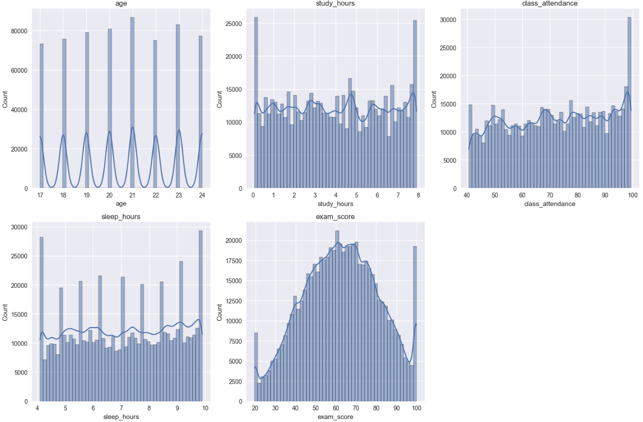
Observation:
This dataset is very clean, data has fairly uniform distribution, target variable exam_score has normal bell-shaped distribution, no obvious outliers, showing data has been well preprocessed or is high-quality synthetic data.
3.4.2. Categorical Variables
Purpose: View frequency of occurrence of groups
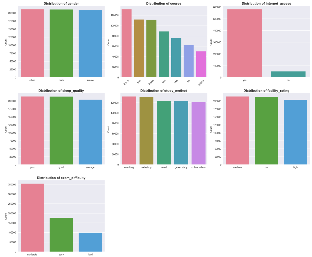
Observation:
Categorical variables show fairly even data distribution in most groups, except internet_access has overwhelming "yes" ratio and exam_difficulty mainly concentrates at "moderate" level.
3.5. Relationship between Features and Target
In this problem, target is numeric variable, so apply Correlation Matrix - Linear correlation to see linear relationship between variables and target.
Linear Correlation (Correlation Matrix)
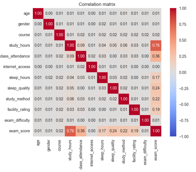
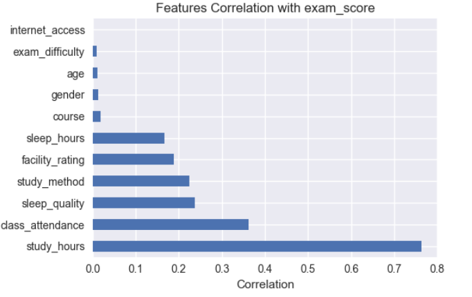
Conclusions from Correlation Analysis
- Correlation analysis mainly reflects linear relationships between features and target variable.
study_hourshas strong linear correlation with target variable (r = 0.76), showing this is an important feature.class_attendance,sleep_qualityandstudy_methodhave weak to moderate linear correlation, suggesting potential non-linear relationships.- Features
age,genderhave almost no linear correlation with target variable. - No serious multicollinearity detected between features.
4. Feature Engineering
In the feature engineering phase, learning behavior variables are transformed and combined to help the model better exploit non-linear relationships in the data.
Principle: "GARBAGE IN - GARBAGE OUT" - Poor data → Poor model
4.1. Remove Unnecessary Features
To ensure removal decisions are accurate, not just based on correlation analysis results from EDA, the team trained a baseline LightGBM model with all features and analyzed Feature Importance and decided to drop the following features:
drop_cols = [
    'id',              # id - does not carry predictive information
    'age',             # Correlation = 0.01 - no impact
    'gender',          # Correlation = 0.01 - no difference
    'internet_access'  # Correlation = 0.00 - no effect
]

df = df.drop(columns=drop_cols, errors='ignore')
for the reasons:
- features have extremely low correlation coefficient (< 0.05) with target variable exam_score as in Correlation matrix
- Feature Importance from baseline model completely aligns with correlation analysis, confirming removal of age, gender, internet_access is correct decision
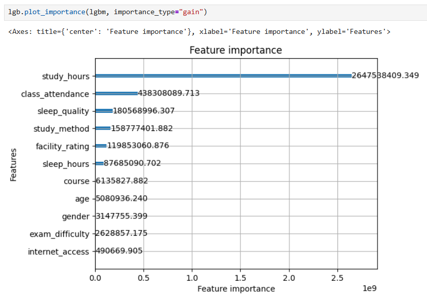
However, still keeping 2 variables exam_difficulty and course because although importance is low, they have business significance.
4.2. Classify and Organize Features
For appropriate handling, we classify features into 3 clear groups:
Group 1: Numerical Features
num_base = [
    'study_hours',       # Study hours per day (0-10h)
    'class_attendance',  # Class attendance rate (0-100%)
    'sleep_hours'        # Sleep hours per day (4-10h)
]
These are continuous variables with strong correlation with target, especially study_hours (r=0.76).
Group 2: Ordinal Categorical (Ordered categorical variables)
cat_ordinal = [
    'sleep_quality',     # Sleep quality: poor < average < good
    'facility_rating',   # Facility rating: low < medium < high
    'exam_difficulty'    # Exam difficulty: easy < moderate < hard
]

# Define clear ordering
sleep_quality_order = ['poor', 'average', 'good']
facility_rating_order = ['low', 'medium', 'high']
exam_difficulty_order = ['easy', 'moderate', 'hard']
These variables have natural logical order, need to be encoded in correct order for model to learn high-low levels.
Group 3: Nominal Categorical (Unordered categorical variables)
cat_onehot = [
    'study_method',  # Study method
    'course'         # Course
]
These variables have no natural order, need One-Hot Encoding to avoid wrong assumptions.
4.3. Building New Features
Based on understanding of education domain and EDA analysis, we created 5 new features to capture complex relationships:
def add_features(df: pd.DataFrame) -> pd.DataFrame:
    """
    Create new features from domain knowledge about learning
    """
    df = df.copy()

    # 1. Binary Indicators - Mark important thresholds
    df['high_study'] = (df['study_hours'] > 6).astype(int)
    df['low_attendance'] = (df['class_attendance'] < 60).astype(int)

    # 2. Interaction Features - Capture combination effects
    df['study_efficiency'] = df['study_hours'] * df['class_attendance']
    df['sleep_attend_product'] = df['sleep_hours'] * df['class_attendance']

    # 3. Deviation Feature - Measure deviation from ideal level
    df['sleep_deviation'] = (df['sleep_hours'] - 7).abs()

    return df
Details of each feature group:
| Group | Feature | Formula / Code | Meaning | Rationale & Explanation | Example |
|---|---|---|---|---|---|
| A. Binary Indicators | high_study |
study_hours > 6 |
Mark students who study a lot (> 6 hours/day) | Create clear threshold for model to identify high-performing student groups. EDA shows clear distinction between > 6h and < 6h groups. | > 6h → 1 < 6h → 0 |
low_attendance |
class_attendance < 60 |
Alert low attendance rate | Identify at-risk student groups. 60% threshold is important dividing point in education system. | < 60% → 1 ≥ 60% → 0 |
|
| B. Interaction Features | study_efficiency |
study_hours × class_attendance |
Comprehensive study efficiency | Combines 2 features with highest correlation (0.76 and 0.36). Study much but not attend regularly → low efficiency; study little but attend regularly also not enough. | A: 8×90% = 720 (high) B: 8×50% = 400 (avg) C: 3×90% = 270 (low) |
sleep_attend_product |
sleep_hours × class_attendance |
Interaction between sleep and attendance | Sufficient sleep helps increase concentration when attending class. This feature captures combined effect between health and class participation level. | Good sleep + regular attendance → high efficiency | |
| C. Deviation Feature | sleep_deviation |
|sleep_hours − 7| |
Deviation from ideal sleep level | Captures U-shaped non-linear relationship. Too little or too much sleep both negatively affect; closer to 7 hours better. | 7h → 0 (optimal) 5h → 2 (sleep deprived) 9h → 2 (oversleep) |
4.4. Encoding for Numerical and Categorical Variables
Step 1: StandardScaler for Numerical Features
('num', StandardScaler(), num_features)
- Formula:
z = (x - mean) / std - Result: Mean = 0, Std = 1
- Reason for use:
- Although LightGBM (tree-based) is not sensitive to scale, StandardScaler is still necessary because:
- Ensures pipeline consistency
- Stabilizes distribution of features created from multiplication (study_efficiency, sleep_attend_product)
- Helps fair comparison if testing with other models (Linear, SVM)
- Interaction features have very large range (e.g., 8×90=720) compared to binary features (0-1) → Scaling helps balance
Step 2: OrdinalEncoder for Ordinal Features
('ord', OrdinalEncoder(
    categories=[sleep_quality_order, facility_rating_order, exam_difficulty_order]
), cat_ordinal)
- Encoding:
sleep_quality: poor → 0, average → 1, good → 2facility_rating: low → 0, medium → 1, high → 2exam_difficulty: easy → 0, moderate → 1, hard → 2- Reason: Preserves logical order, model learns high-low levels (poor < average < good)
Step 3: OneHotEncoder for Nominal Features
('onehot', OneHotEncoder(
    drop='first', handle_unknown='ignore', sparse_output=False
), cat_onehot)
- Result:
study_method(3 categories) → 2 binary columnscourse(5 categories) → 4 binary columns- Important parameters:
drop='first': Remove first category to avoid multicollinearity (dummy variable trap)handle_unknown='ignore': If test set has new category → all columns = 0 (safer than error)sparse_output=False: Return numpy array instead of sparse matrix (easier to handle)
5. Model Training
5.1. Data Preparation
from sklearn.model_selection import train_test_split

# Separate features and target
X = df.drop('target', axis=1)
y = df['target']

# Split train/test (80/20)
X_train, X_test, y_train, y_test = train_test_split(
    X, y, test_size=0.2, random_state=42
5.2. Models Used
| Model | Model Type | Advantages | Disadvantages | When to Use |
|---|---|---|---|---|
| Linear Regression (Baseline) | Linear | Simple, easy to understand, fast training | Assumes linear relationship, sensitive to outliers, prone to overfitting | Use as baseline for comparison |
| Ridge Regression (L2) | Linear | Reduces overfitting, handles multicollinearity well | Does not automatically remove features | When many highly correlated features |
| Lasso Regression (L1) | Linear | Automatic feature selection (zeroes coefficients), reduces overfitting | Not stable when features strongly correlated | When need to eliminate unimportant features |
| LightGBM | Tree-based (non-linear) | Lighter and faster than XGBoost, handles large data well, learns non-linear relationships and feature interactions | Harder to interpret than linear models | When data is complex, non-linear relationships, need high performance |
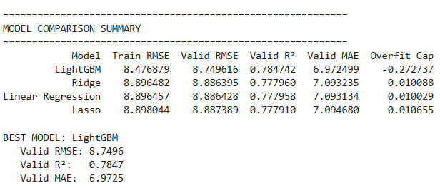
LightGBM was chosen as the final model for achieving best performance on validation set, stable generalization capability and approaching Kaggle leaderboard top results. This result proves Feature Engineering and Model Selection pipeline is reasonable for the problem.
Comparison with Kaggle leaderboard:
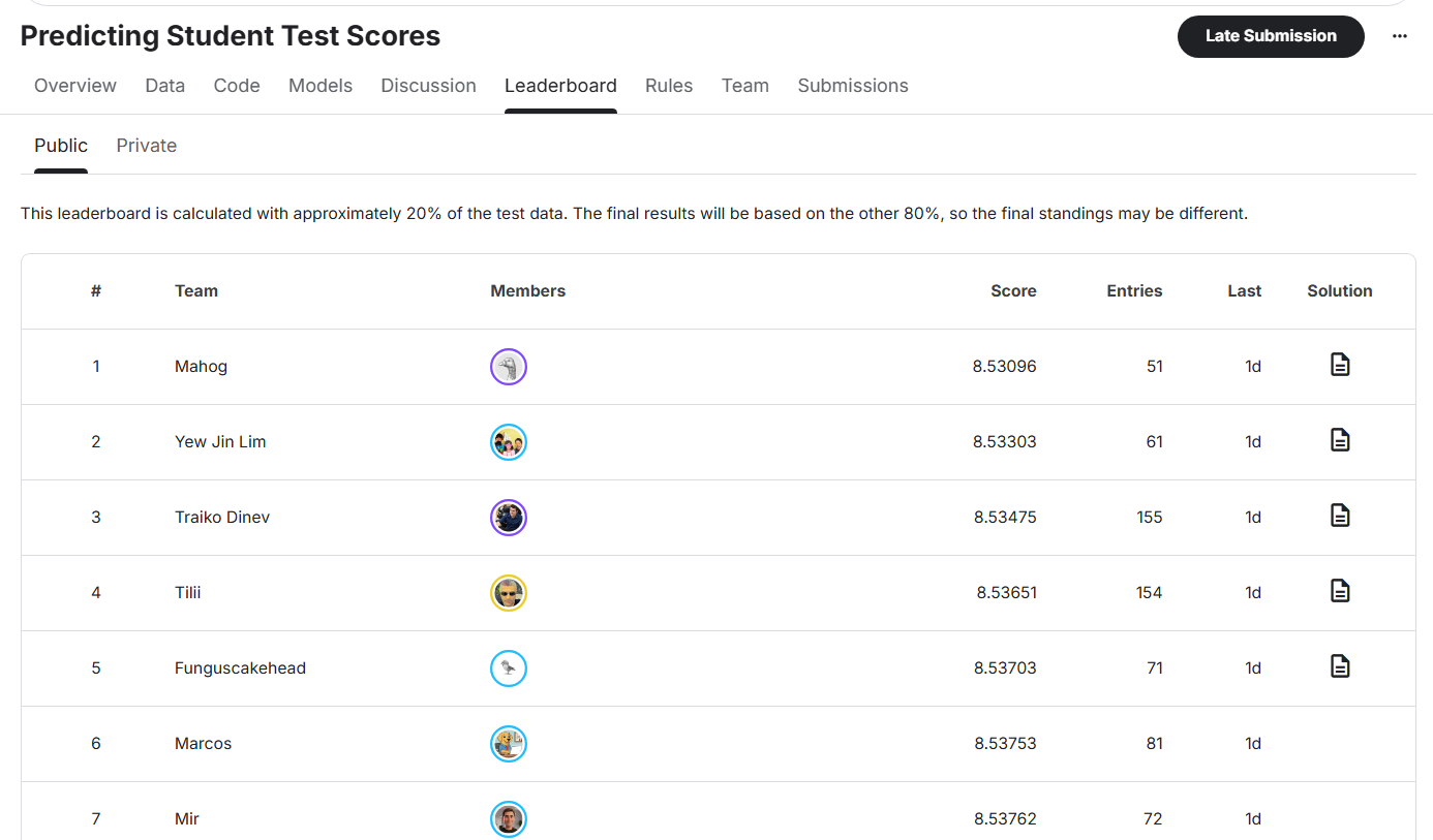
Current best result for this problem on Kaggle achieves approximately RMSE ≈ 8.53x.
LightGBM model in project achieves RMSE ≈ 8.75, only about 0.22 RMSE behind.
6. Model Deployment with Gradio
After training, the LightGBM model is used to build a simple prediction application using Gradio.
Users input information such as:
- Study time
- Attendance level
- Sleep
- Study method

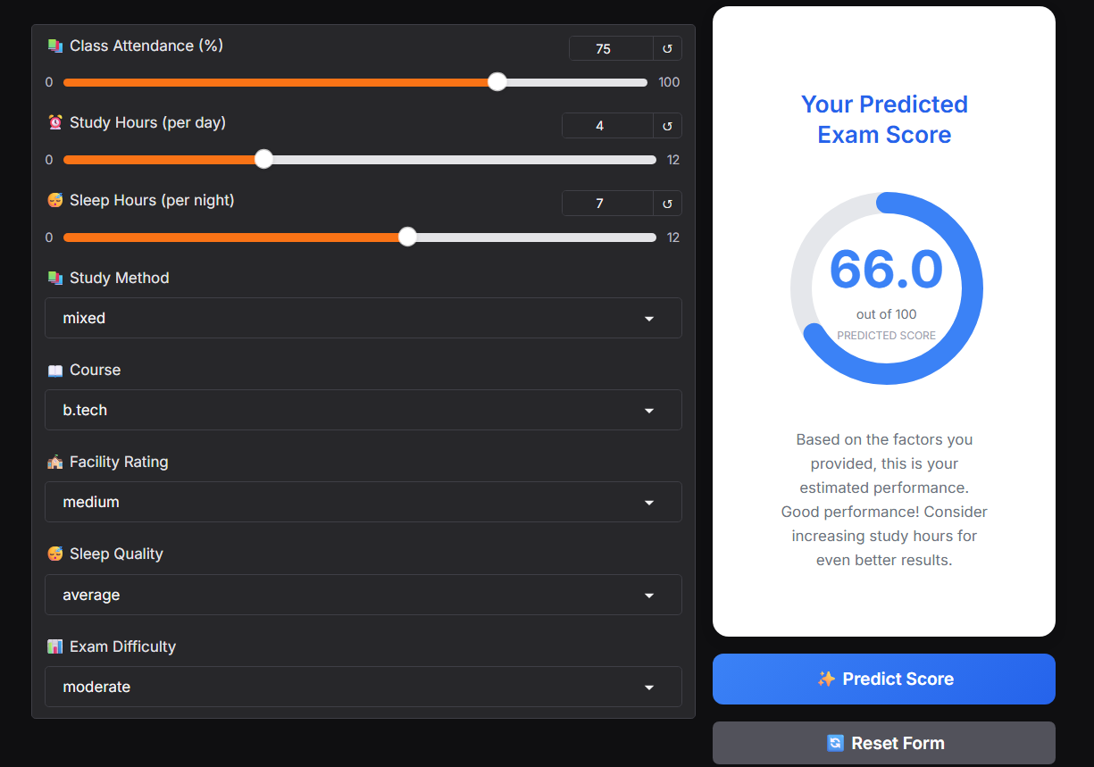
Input data is processed through the same Feature Engineering pipeline used during training. The model returns corresponding predicted score.
Conclusion
In this article, we built a complete Machine Learning pipeline for the exam score prediction problem, starting from EDA, Correlation Analysis, Feature Engineering to Model Training and Evaluation.
Results show:
- Study behavior features (study hours, attendance, sleep) play the most important role in predicting learning outcomes.
- Linear models (Linear, Ridge, Lasso) are suitable as baselines thanks to simplicity and easy interpretation, but limited when data has non-linear relationships.
- LightGBM excels thanks to ability to exploit interactions and non-linearity, achieving RMSE ≈ 8.75, approaching Kaggle top results (~8.54).
In the future, the model can be further improved through cross-validation, deeper hyperparameter tuning and ensemble methods. However, within current problem scope, the pipeline is complete enough to deploy with Gradio and use as a practical ML project for portfolio.
Chưa có bình luận nào. Hãy là người đầu tiên!