
(Note: All illustrations and diagrams in this article are AI-generated by Gemini.)
In Blog 1, we together "decoded" derivatives and Gradient. We understood that derivatives tell us "when the input changes a tiny bit, how will the output vary". And Gradient, simply a vector gathering partial derivatives together, acts like a compass pointing to the direction of fastest change for a function.
But the question arises: What is this compass used for in practice?
In Machine Learning, Gradient is not just a dry mathematical concept. It is the "engine" powering one of the most powerful techniques today: Gradient Boosting — a method that uses Gradient to continuously "learn from past mistakes".
However, to truly master Gradient Boosting or other complex algorithms, we need to understand a broader philosophy: Ensemble Learning.
I. Ensemble Learning
1.1 The Power of the Crowd
Imagine you're wandering into a bustling fair, and right in front of you is an interesting challenge: a giant glass jar filled with candies. The organizer poses a simple but tricky challenge: "Whoever guesses the correct number of candies in the jar wins!".
You squint your eyes, trying to estimate... 800 pieces? Or maybe 1200? It's really hard to give an exact number just by looking. At this moment, you turn to ask the people around you. One person beside you firmly says 500, while another guesses up to 2000. Clearly, each individual can be very far off from reality, some guessing too high, others too low.
But here's the magical thing about mathematics and statistics: If you ask 100 people and calculate the average of all those answers, the resulting number is often astonishingly accurate — it's closer to the actual number of candies than any individual's prediction!
Why does this phenomenon occur? It's because each person carries their own random error. When we perform the averaging calculation, these errors cancel each other out, leaving only the "correct signal" accumulated. This phenomenon is called the Wisdom of the Crowd, and this is exactly the foundational philosophy behind Ensemble Learning.
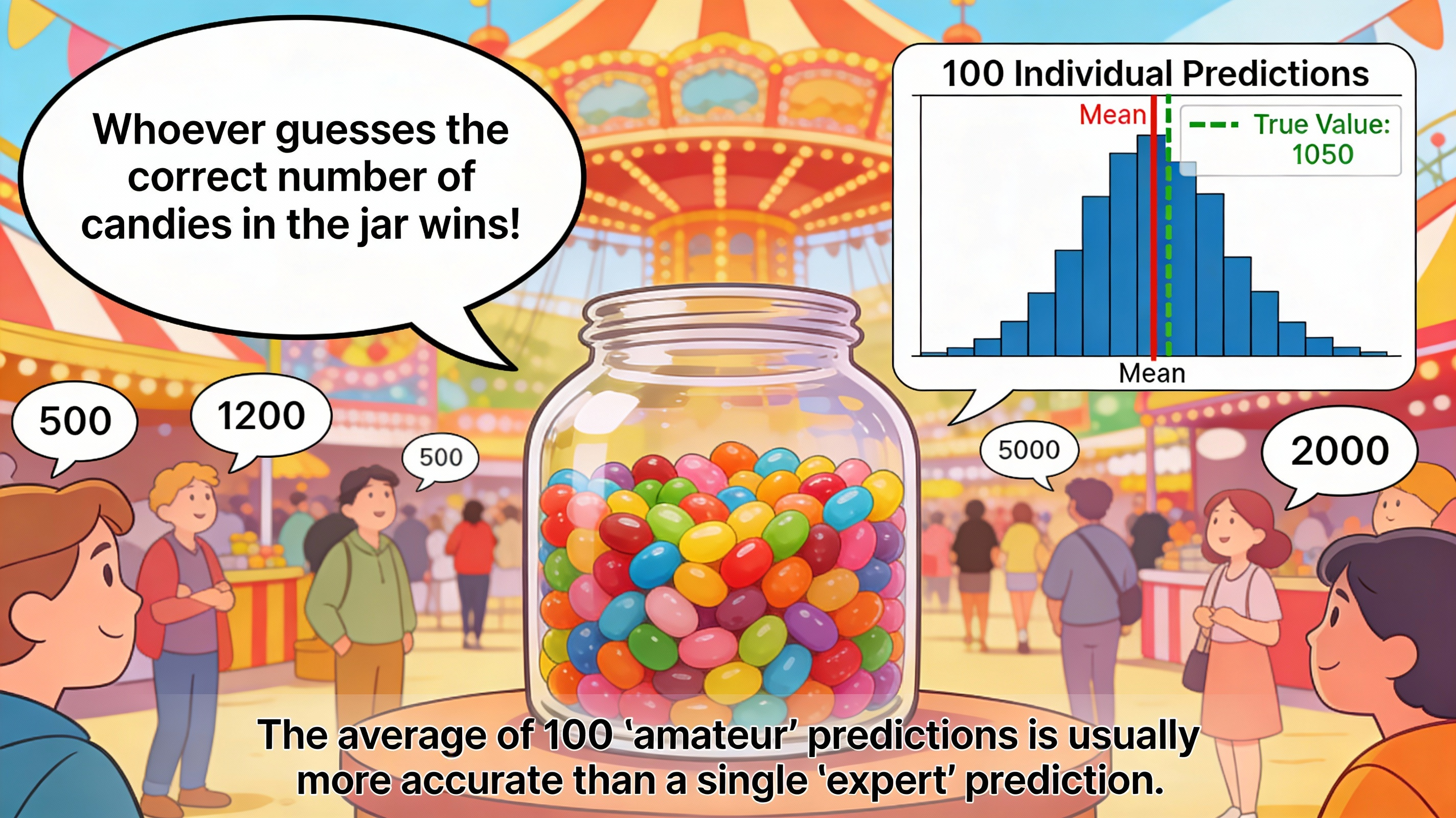
Figure 1. The average of 100 "amateur" predictions is often more accurate than 1 single "expert" prediction
1.2 What is Ensemble Learning?
In the world of Machine Learning, Ensemble Learning is a method of combining multiple machine learning models together to solve a problem. These component models are often called weak learners. Our goal is to combine their strengths to create a strong learner that is superior.
Each individual model, like a person guessing candies, may not be perfect and prone to making mistakes. However, when combined intelligently, individual errors are "leveled out", helping the final result become more stable and accurate.
If we go back to the candy jar example above, we can visualize it as follows:
- Each person guessing candies: Corresponds to a weak learner (prediction may be wrong, not optimal).
- Group of 100 people: Corresponds to an ensemble (collection of models).
- Average value of predictions: This is the strong learner (final result with higher accuracy).
1.3 Two Major Schools of Thought: Bagging and Boosting
Although they share the common purpose of combining models, in Ensemble Learning there exist two very different schools of thought about how to implement it: Bagging and Boosting. Their difference lies in how models are built and connected to each other.
1.3.1 Bagging (Bootstrap Aggregating)
Imagine you're the director of a large corporation and need to decide whether to invest in a new project. You summon 10 top analysts, each skilled but with their own unique perspectives and viewpoints.
With this approach, you give each expert a slightly different set of documents (all taken from the original data, but randomly selected). Each expert works independently in their own room, no one communicates with anyone else. Finally, you aggregate opinions by having them vote (Voting) or taking the average (Averaging). This method helps diversify perspectives and eliminate individual errors.
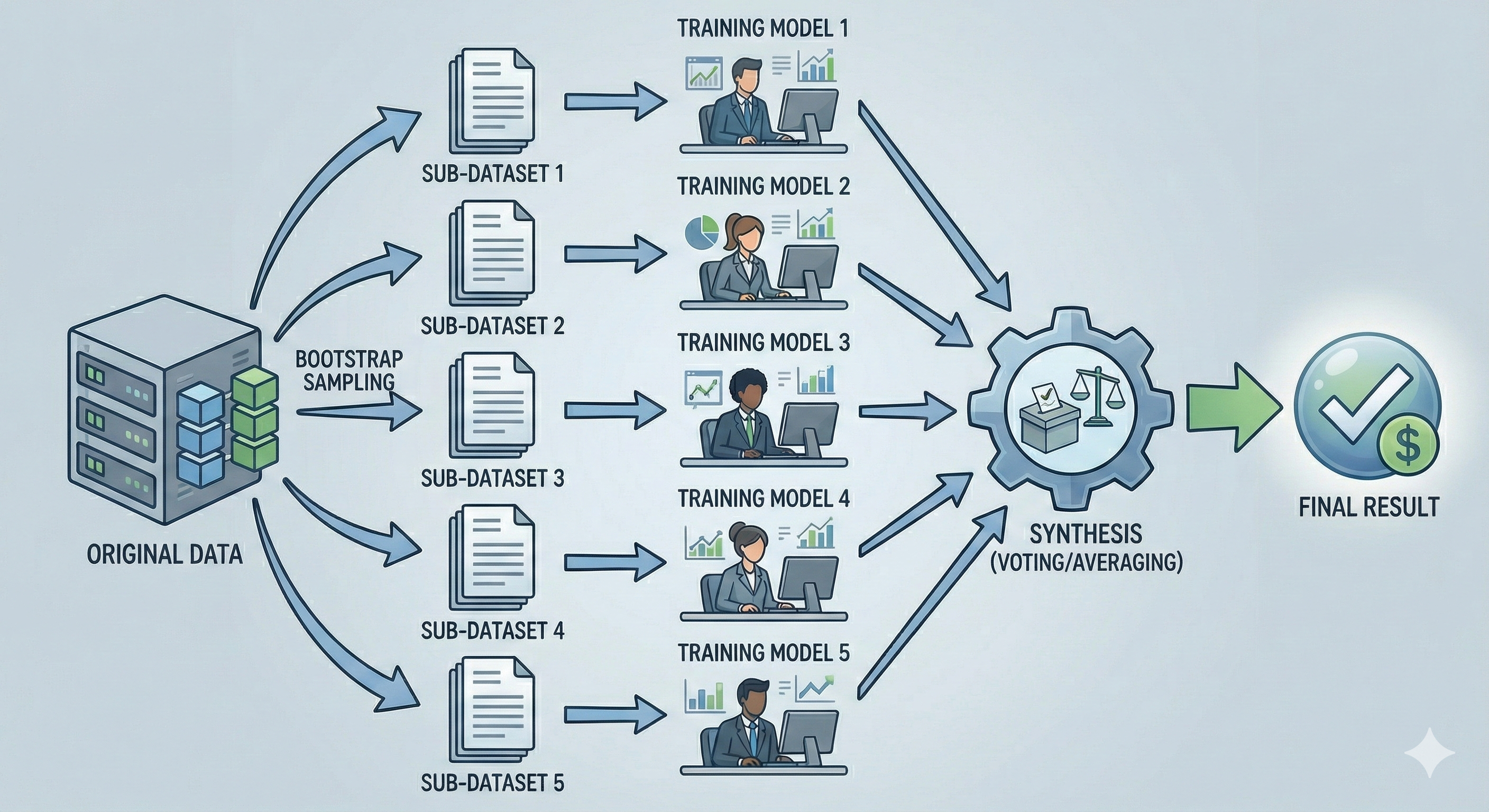
Figure 2. Bagging creates diversity by having models learn from different data then aggregating.
Technical Definition:
Technically, Bagging operates through 3 main steps:
-
Step 1 — Bootstrap Sampling: From the original dataset, we create multiple "copies" by randomly selecting data points (with replacement). Statistics show that each bootstrap sample contains about 63% of the original data, the remainder is called Out-of-Bag samples.
-
Step 2 — Parallel Training: Each sub-model is trained independently on a bootstrap sample. These models completely don't "know" about each other's existence.
-
Step 3 — Aggregating: The final result is decided by majority voting (for classification problems) or averaging (for regression problems).
The ultimate goal of Bagging is to reduce Variance, helping the model become more stable and less sensitive to noise. The most representative example of this school is Random Forest.
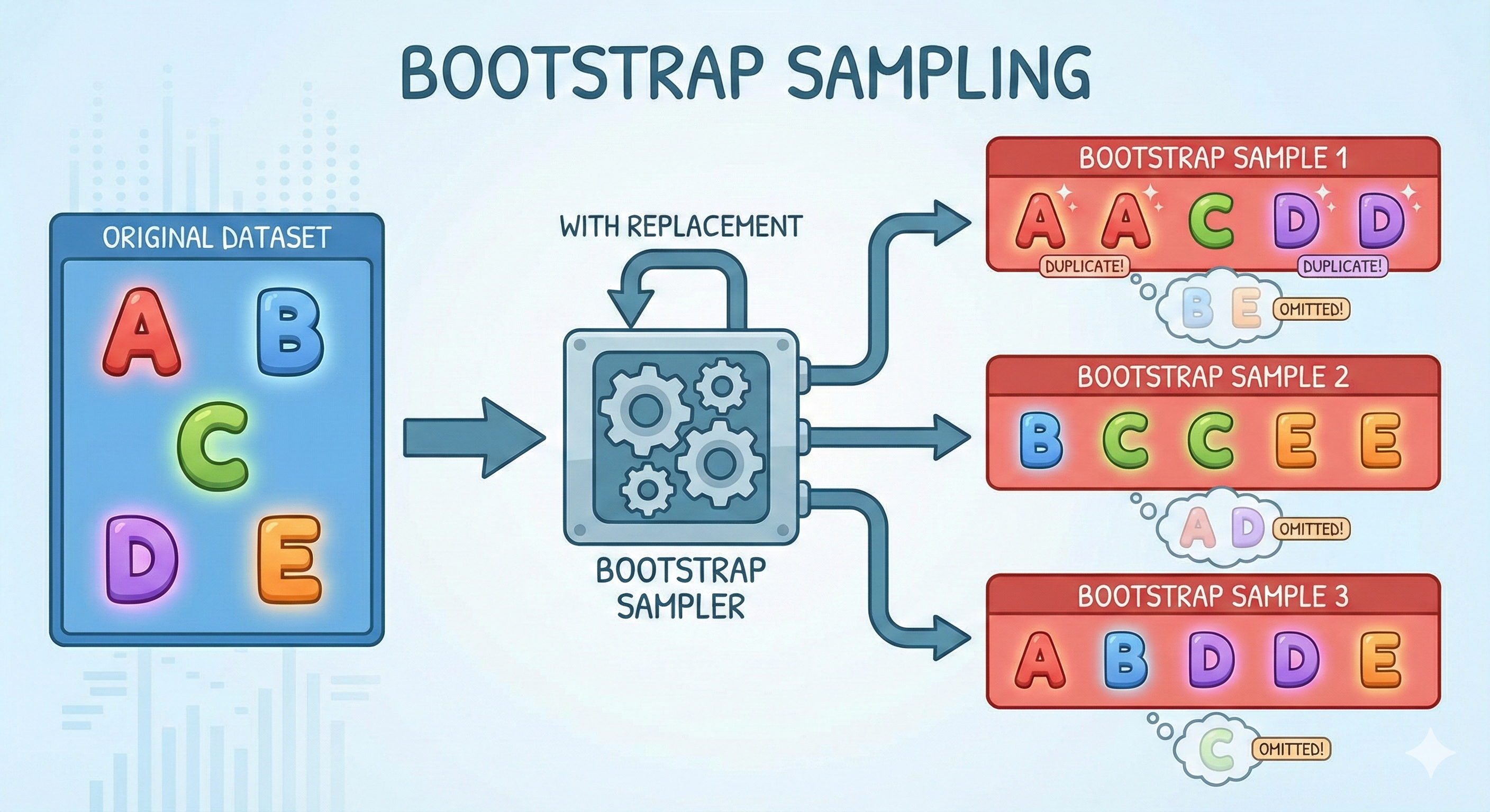
Figure 3. Bootstrap sampling creates diverse datasets from the same original source.
1.3.2 Boosting
Still the same company, but this time you apply a completely different management strategy. You assign the project to the first expert to handle first. He produces a report, but of course there are still some errors or uncertainties.
Instead of ignoring them, you mark these errors and hand them to the second expert with clear instructions: "Focus on fixing the parts that the previous person got wrong". The second expert finishes, but there are still some small errors. You pass it on to the third expert to continue fixing... And so on, each successor learns from the predecessor's mistakes. This is the sequential way of working.
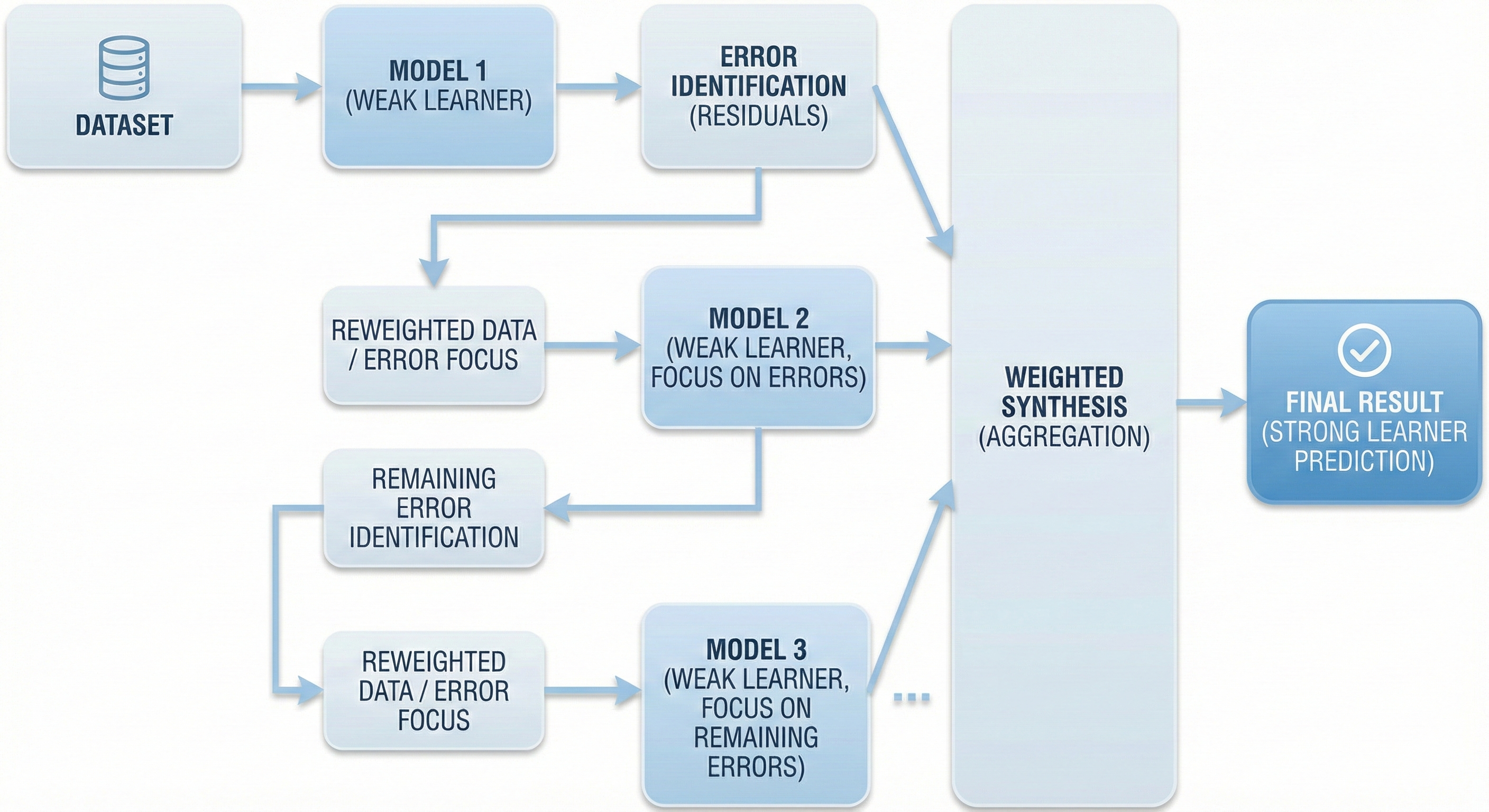
Figure 4. Boosting trains sequentially, later models focus on fixing previous models' errors.
Technical Definition:
Boosting operates based on the principle of sequential learning:
-
Step 1: Train the first model on the entire dataset.
-
Step 2: Identify the data points that the model predicted incorrectly (called Residuals).
-
Steps 3 & 4: Train the next model, but force it to focus on those wrong points (by increasing weights or learning directly on residuals). This process repeats continuously.
-
Step 5: The final result is a weighted combination of all models in the chain.
If you still remember the concept of Gradient from the previous blog post, then in Gradient Boosting, the "mistakes to fix" are identified by the derivative (Gradient) of the loss function. Each new model generated tries to follow the direction of fastest error reduction (negative gradient). The main goal of Boosting is to reduce Bias. Famous representatives of this school include XGBoost, LightGBM, and CatBoost.
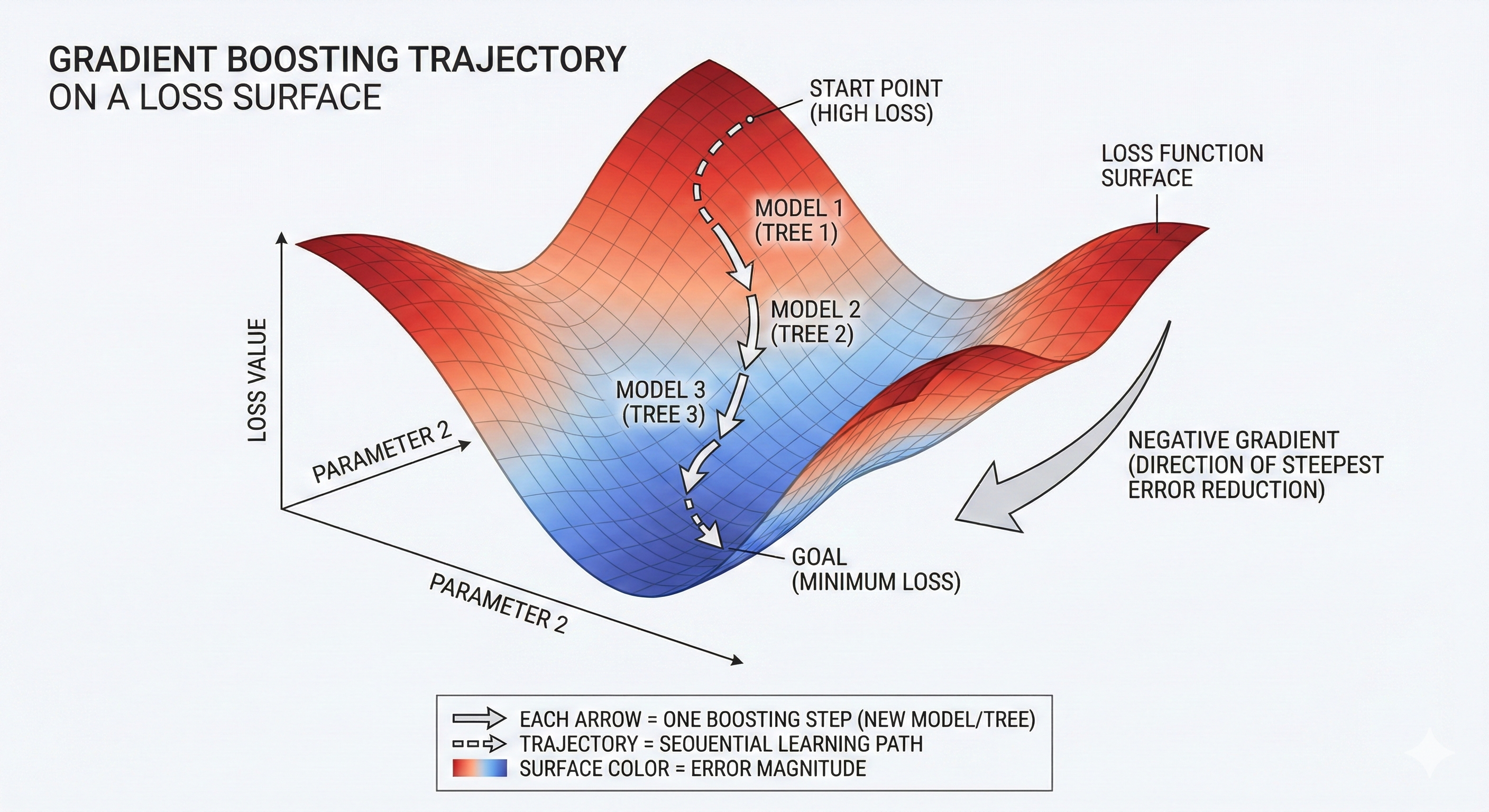
Figure 5. Each tree is a downhill step helping reduce Loss fastest.
1.4 Comparing Bagging and Boosting
To easily visualize the difference between these two "giants", let's look at the comparison table below:
| Feature | Bagging (Bootstrap Aggregating) | Boosting |
|---|---|---|
| Training method | Parallel – Models are independent of each other | Sequential – Later models depend on previous models |
| What does the model learn from? | Random Bootstrap samples | Residuals of the previous model |
| Main goal | Reduce Variance | Reduce Bias |
| Overfitting risk | Low (due to averaging mechanism) | Higher (if trained too thoroughly will learn noise too) |
| Representative examples | Random Forest | XGBoost, LightGBM, CatBoost |
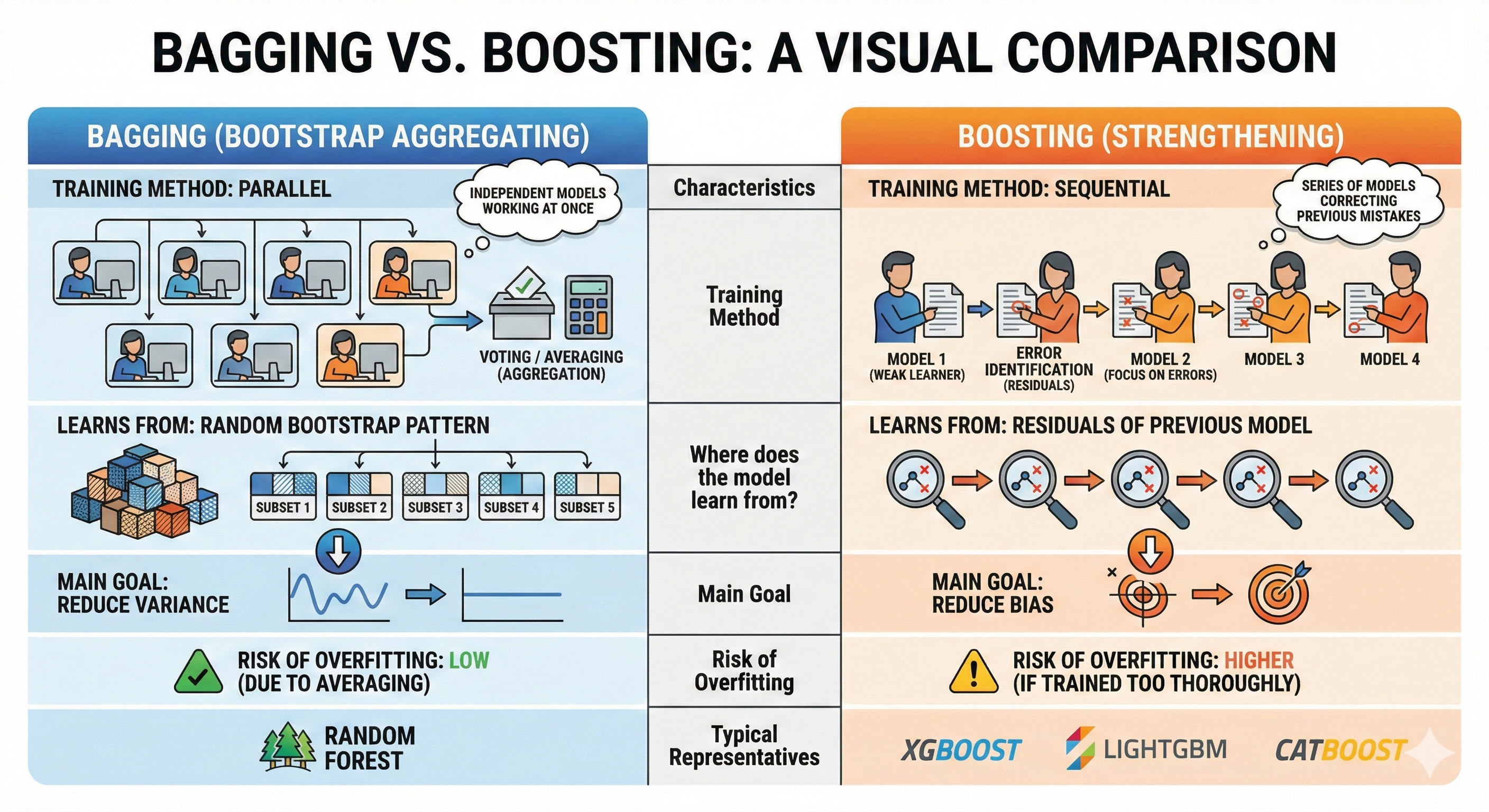
Figure 6. Bagging works in parallel; Boosting works sequentially and corrects errors.
1.5 Models We Will Explore
In this series of articles, we will dive deep into 3 models in evolutionary order from simple to complex:
1.5.1. Decision Tree:
This is the first foundational brick. It's the simplest, easiest to understand model, but it's also the component that makes up more complex algorithms. Understanding Decision Tree is a mandatory prerequisite for you to understand why we need Ensemble.
1.5.2. Random Forest:
An excellent representative of the Bagging school. As the name suggests, this is a "forest" made up of hundreds of decision trees. This combination creates an extremely robust model, less prone to overfitting and especially very easy to use because it doesn't require too much parameter tuning.
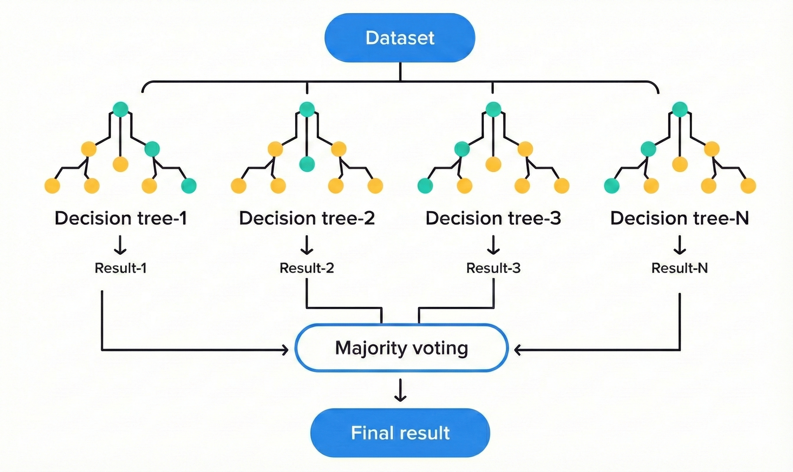
Figure 7. Random Forest combines the power of trees using the voting method.
1.5.3. XGBoost (Extreme Gradient Boosting):
Representative of Boosting and the "heavy weapon" in Data Science competitions. XGBoost uses Gradient to optimize the sequential learning process, continuously correcting errors to achieve extremely high accuracy. However, great power comes with great responsibility: it needs to be tuned carefully to avoid rote learning (overfitting).

Figure 8. XGBoost consists of a chain of trees learning from previous trees' mistakes.
1.6 Why Understand All Three?
You might wonder: "If XGBoost is that powerful, why not learn it directly instead of taking the long way?". The answer lies in understanding the essence of the problem.
The journey from Decision Tree to XGBoost is a logical story about solving each model's weaknesses:
- Decision Tree helps you understand the "divide and conquer" mechanism, but it suffers from "large fluctuations" (high variance).
- Random Forest was born to cure the "fluctuation" disease by using Bagging to diversify.
- XGBoost continues one more step to cure the "inaccuracy" disease (bias) by using Boosting to thoroughly correct errors.
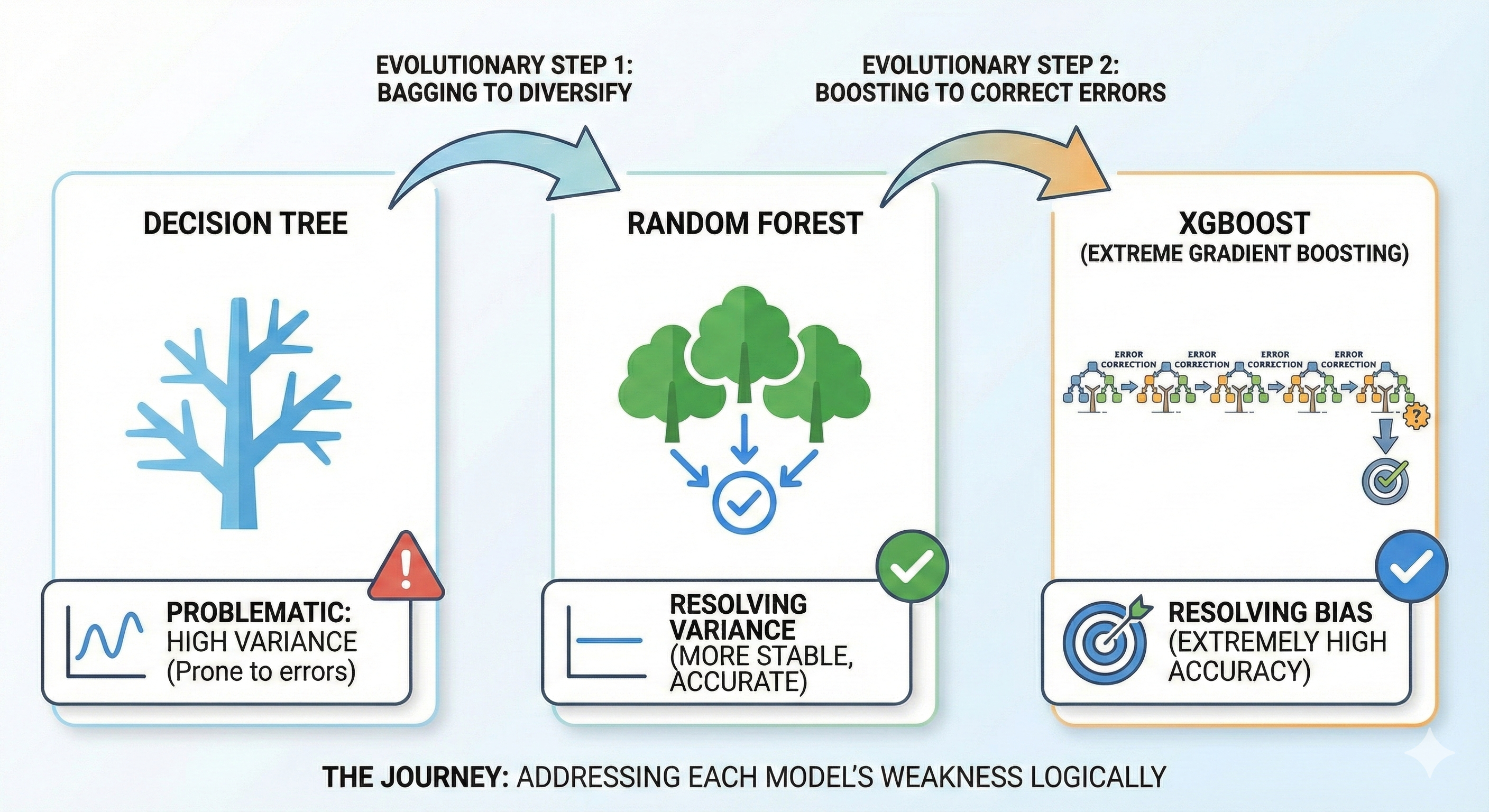
Figure 9. The journey of addressing weaknesses from Decision Tree to XGBoost.
1.7 Five Analytical Lenses
To truly master these models, we won't just learn dry theory. For each model, I will analyze them with you through 5 important aspects — like examining a diamond under 5 different angles of light:
- Hyperparameters: Which "knobs" are most important to control the model?
- Feature Engineering: What kind of data does this model like? How should features be processed?
- Validation: How to evaluate the model fairly?
- Overfitting: What signs show the model is "rote learning" and how to prevent it?
- Bias-Variance Tradeoff: Where does this model stand in this classic balancing problem?
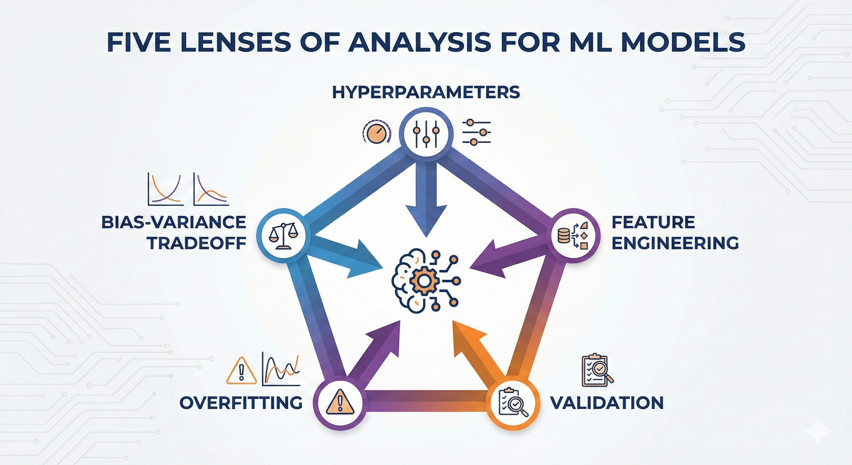
Figure 10. Each model is comprehensively evaluated through 5 optimization lenses.
II. Five Analytical Lenses for Models
2.1 Hyperparameters
Imagine you're cooking a pot of beef pho. During cooking, you taste the broth, if it's bland you add salt, if it's not sweet enough you add more bones. The seasonings you adjust while cooking to achieve the best taste, that's the "learning" process.
However, there are decisions you must make before turning on the stove: Will you use a pressure cooker or a regular pot? How long do you plan to simmer the bones (2 hours or 8 hours)? Do you keep the heat high or low? These decisions definitely affect the final bowl of pho, but you can't change the pot while cooking. Those initial settings are Hyperparameters.
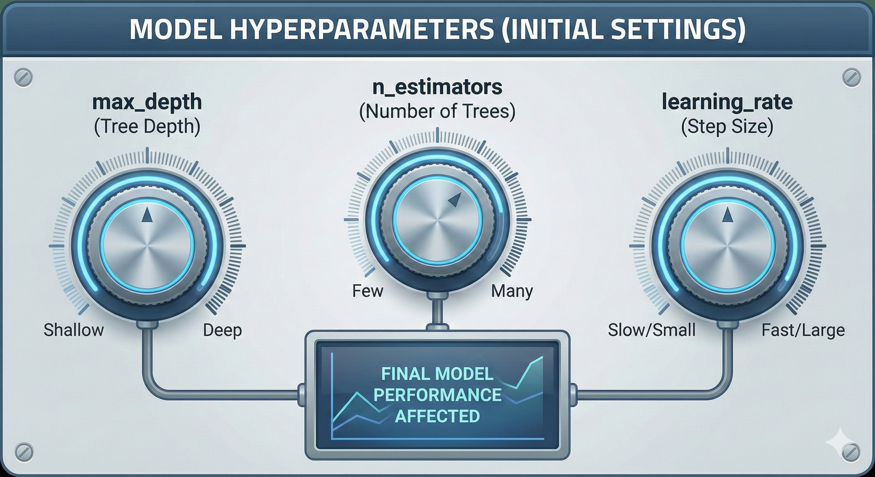
Figure 11. Hyperparameters are adjustment knobs that help optimize model operation.
Definition:
In Machine Learning, Hyperparameters are the "adjustment knobs" that you must set manually before the training process begins. The model cannot learn them from the data itself.
We need to clearly distinguish from Parameters:
- Parameters: What the model learns and adjusts itself during training (e.g., weights in neural networks, or split thresholds in decision trees - like tasting and adding salt).
- Hyperparameters: What you set up initially (e.g., tree depth, number of trees in the forest - like choosing the pot and simmering time).
Below are some important hyperparameters we will frequently encounter:
| Hyperparameter | Meaning | Commonly found in |
|---|---|---|
| max_depth | Limits how many times the tree is allowed to "split" (deeper trees are more complex). | Decision Tree, RF, XGBoost |
| n_estimators | Number of sub-trees in a "forest" (ensemble). | Random Forest, XGBoost |
| learning_rate | The degree of contribution/correction of each new tree to the overall result. | XGBoost, Gradient Boosting |
| min_samples_split | Minimum number of samples required to continue splitting a branch. | Decision Tree, RF, XGBoost |
2.2 Feature Engineering
Imagine you're teaching a child to recognize dogs through pictures. If you only show the child raw data in the form of tiny pixels with millions of color numbers, the child will find it very difficult to learn what a dog is.
But if you point and say: "Look, it has 4 legs", "it has a long tail", "it has fluffy fur", the child will recognize it much faster. Your conversion from meaningless pixels to concepts like "legs", "tail", "fur" is Feature Engineering. You're helping the model "see" the problem more easily.
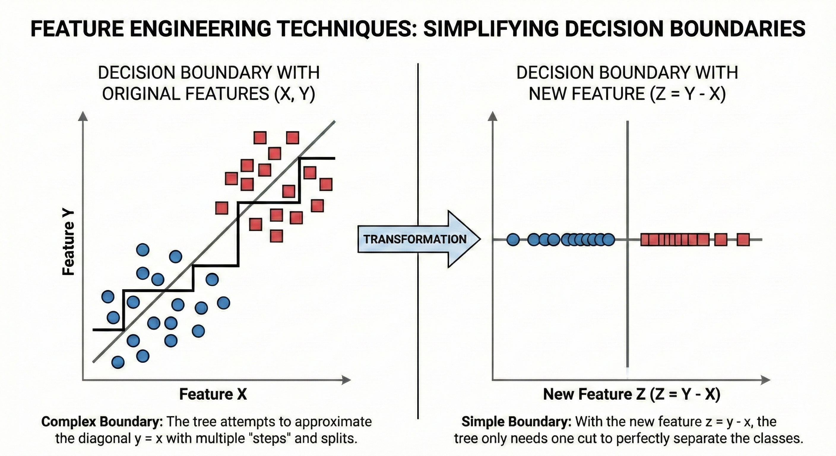
Figure 12. Feature Engineering helps tree models recognize patterns more easily.
Definition:
Feature Engineering is the process of creating, selecting, and transforming features from raw data to help the model learn more effectively. This is the most important bridge between raw data and algorithms.
Especially for Tree-based models, this technique is extremely important because of their inherent weakness:
- Trees can only create cuts perpendicular to axes (horizontal or vertical).
- If the data's pattern is a diagonal line ($A \times B$ or $A / B$), the tree will have to create many small stair steps to approximate that diagonal (very expensive and inefficient).
- However, if you pre-create a new feature $C = A \times B$, the tree only needs exactly one cut and it's done!
2.3 Validation
Remember back to school days, when you were studying for university entrance exams. If you only focused on doing the same old test papers over and over and memorizing the answers (A, B, C, D), you would definitely get perfect scores on those papers. But when entering the real exam room, encountering a brand new paper, you would easily "slip on a banana peel" and fail.
To avoid this situation, you usually set aside a few practice tests that you've never seen before to self-check close to exam day. If you do well on these practice tests too, it means you've truly understood the material rather than just rote memorizing. That "practice test" process is Validation.
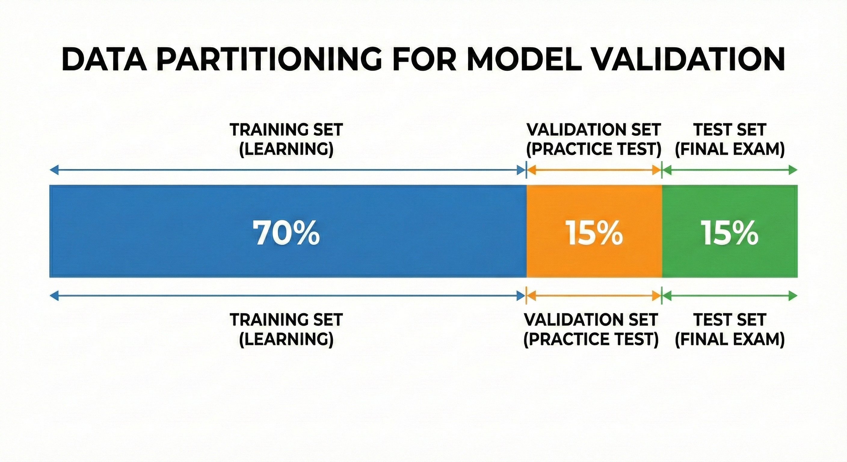
Figure 13. Proper data splitting helps accurately evaluate the model's generalization ability.
Definition:
Validation is the process of evaluating a model's performance on a dataset it has never seen during training. The core goal of Machine Learning is not to "memorize" old data, but to generalize to predict correctly on new data.
In practice, we usually divide data into 3 parts:
- Training set: The textbook for the model to learn knowledge.
- Validation set: Practice tests to preliminarily evaluate and tune hyperparameters.
- Test set: The real exam, used only once at the very end to finalize results.
2.4 Overfitting
Suppose you're teaching a computer to recognize handwritten digits. In your training dataset, coincidentally all the people who wrote the number "7" were left-handed, so every 7 leans slightly to the left.
A model that is "overfitting" will learn mechanically that: "If it's the number 7, it must lean left". The consequence is that when encountering a 7 written straight or leaning right in reality, it will judge: "This is not the number 7!". The model has learned random things (noise) instead of the essence of the number.
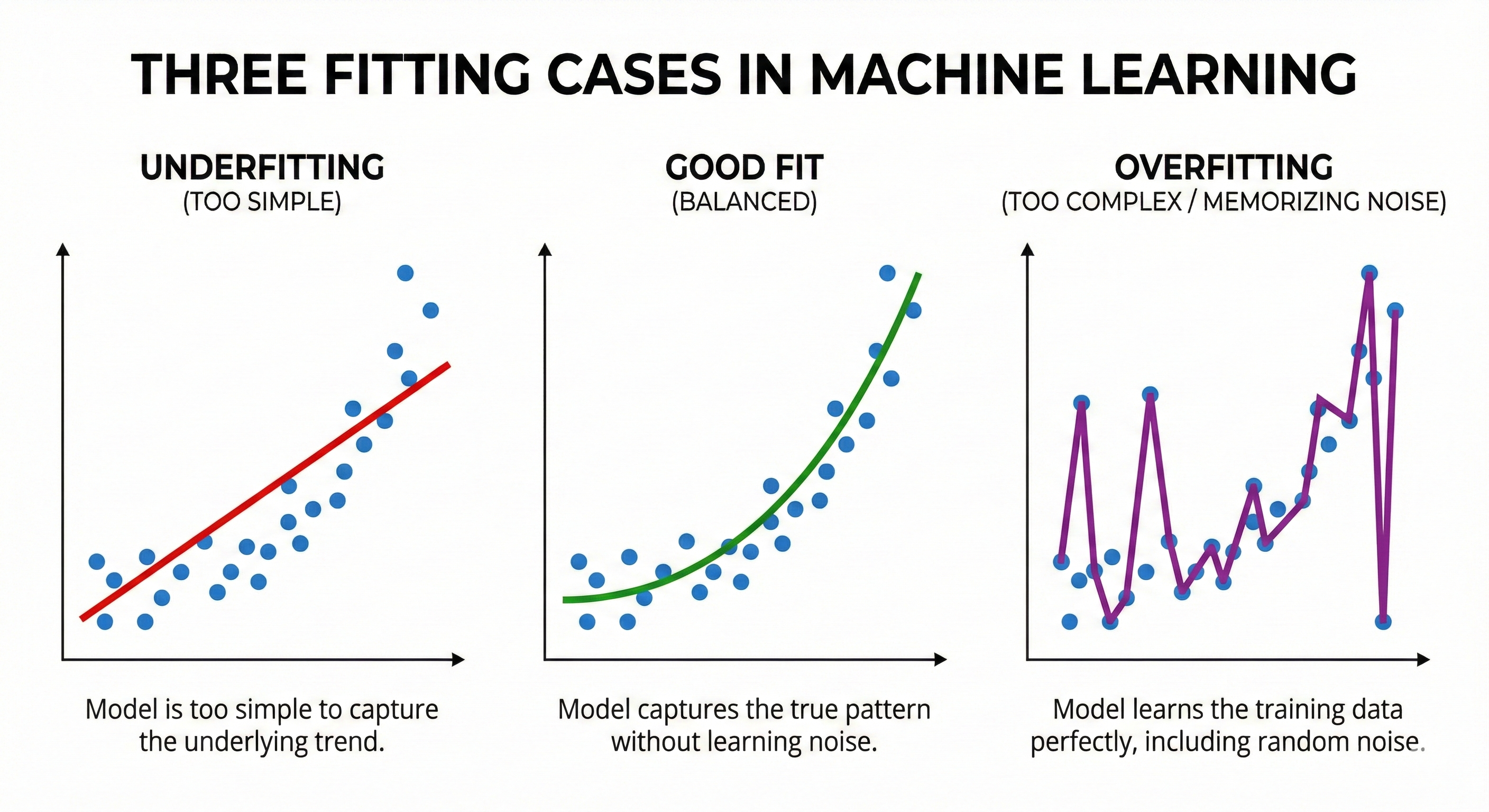
Figure 14. Underfitting is too simple, Overfitting is too complex, Good fit is just right.
Definition:
Overfitting occurs when a model is too complex, to the point where it "memorizes" even the noise in the training set.
Signs to recognize: The score on the Training set is extremely high (nearly perfect), but the score on the Validation/Test set is terribly low. The gap between these two scores, the larger it is, the more severe the overfitting.
The opposite is Underfitting: Occurs when the model is too simple (like a superficial learner), unable to capture the patterns in the data. In this case, scores on both Train and Validation sets are low.
2.5 Bias-Variance Tradeoff
Imagine model training is like target shooting.
-
Case 1 (High Bias): You have very steady hands (stable), but your eyes are crossed so you always aim off to the left. Result: The bullets cluster in one spot, but that spot is far outside the 10-point ring. This is "aiming wrong".
-
Case 2 (High Variance): You aim very accurately at the center, but your hands shake uncontrollably. Result: The bullets fly scattered all around the target, sometimes hitting, sometimes missing. This is "shaky hands".
Goal: We want someone who aims accurately and has steady hands (Low Bias, Low Variance).
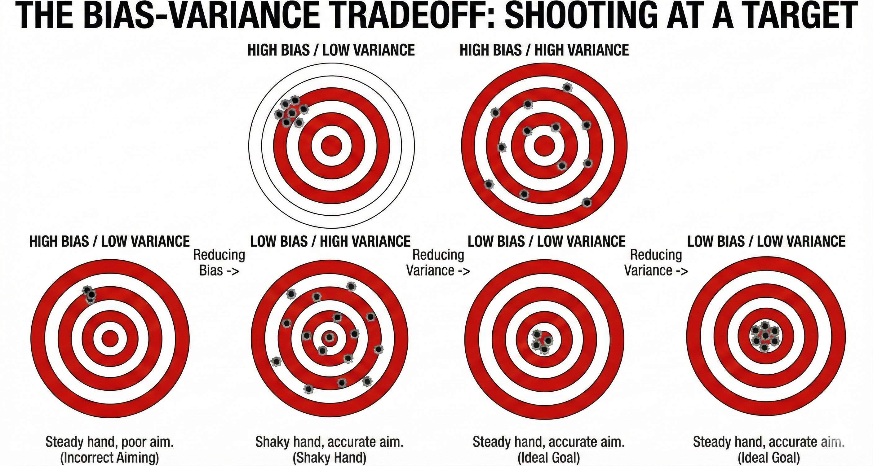
Figure 15. Bias is aiming wrong, Variance is shaky hands; need to aim correctly and steadily.
Definition:
In Machine Learning, there's always a classic tradeoff:
- Bias: Error due to a model that's too simple, unable to learn patterns (Underfitting).
- Variance: Error due to a model that's too sensitive to specific training data, changing the data a little and the result changes dramatically (Overfitting).
Why is it called a Tradeoff? Because it's very difficult to reduce both at the same time.
- Model too simple -> High Bias, Low Variance.
- Model too complex -> Low Bias, High Variance.
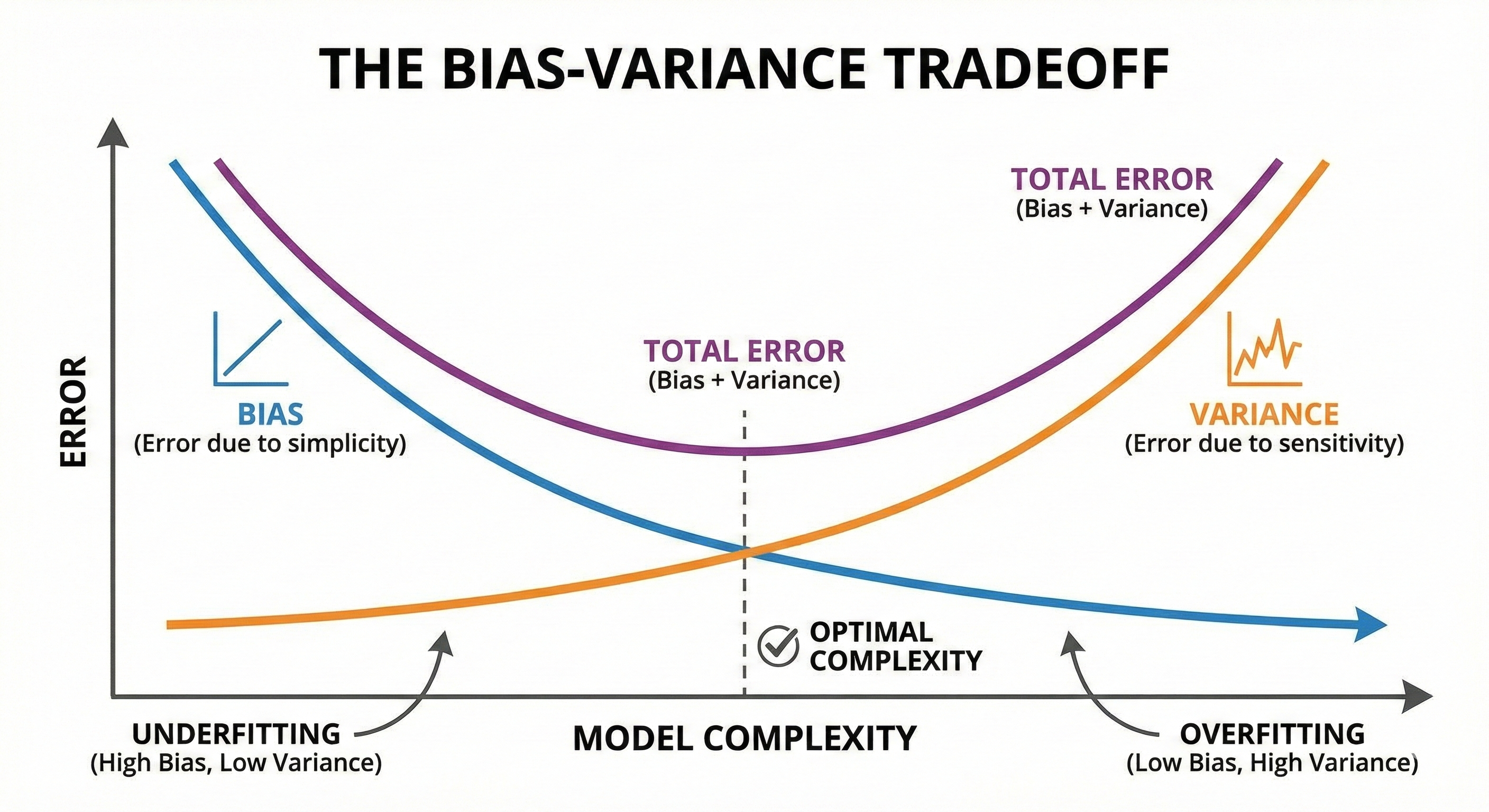
Figure 16. The optimal point is where Bias and Variance are balanced.
The art of the modeler is finding the sweet spot — where the model is complex enough to understand the problem, but simple enough not to rote learn. Ensemble Learning methods (like Bagging and Boosting) were created precisely to solve this balancing problem.
III. Decision Tree
3.1 Introduction to Decision Tree
What is a Decision Tree?
Remember the childhood game "20 Questions". You think of an animal in your head, and the opponent has to guess it by asking Yes/No questions.
- "Does it have 4 legs?" → Yes. (Eliminate chickens, ducks, fish...)
- "Does it bark woof woof?" → No. (Eliminate dogs)
- "Does it like to catch mice?" → Yes.
- "Ah, it's a cat!"
Each question helps you narrow down the space of possible answers, gradually eliminating wrong options until only the most correct option remains. Decision Tree works exactly the same way. It's a machine learning model that makes predictions by performing a series of questions to classify data.
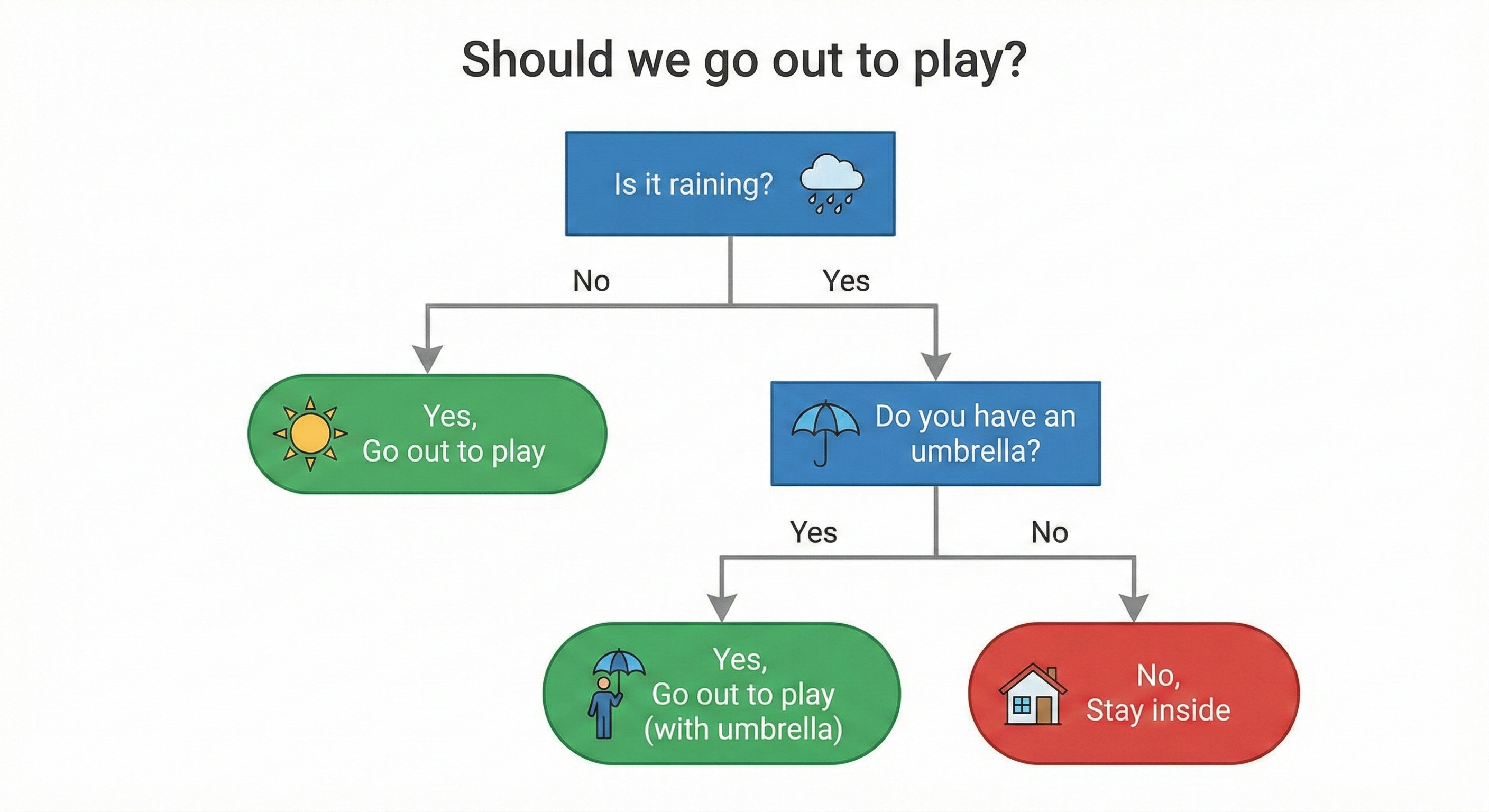
Figure 17. Decision Tree makes decisions through a series of Yes/No questions.
To speak a bit of "technical language", we have the following terms:
- Root node: The first question, where all data begins.
- Decision/Internal node: Subsequent questions at the child branches.
- Leaf node: The final stopping point, where the model makes a prediction.
- Depth: The maximum number of questions the model must go through from root to leaf.
How Decision Tree "learns"
How does the tree know which question to ask first? Why ask "does it have 4 legs" first instead of "what color is it"?
The tree's goal is to choose the question (split) that best separates the data. "Best" here means that after splitting, the resulting child groups must be more "pure" (homogeneous) than the parent group. For example, if a group contains only cats, that group has high purity.
To measure this purity, Decision Tree uses specific mathematical formulas:
- Gini Impurity or Entropy/Information Gain: Used for Classification problems.
- MSE (Mean Squared Error) or Variance: Used for Regression problems.
3.2 Hyperparameters of Decision Tree
As mentioned in Part 2, we need to set up the "knobs" before training. With Decision Tree, there are 3 most important knobs that determine the shape of the tree.
max_depth (Maximum Depth)
Back to the 20 Questions game. If you're only allowed to ask exactly 1 question (Depth = 1), it's very hard to guess the correct animal (this is called a "stump" - a truncated tree). You guess randomly, leading to high error (Underfitting).
Conversely, if you're allowed to ask up to 100 questions (Depth = 100), you can ask extremely detailed questions like "Does this animal have a scar on its left leg?". You'll guess that specific animal exactly right, but this knowledge is too detailed and can't be applied to other animals. That's Overfitting.
- Low Depth: Simple tree → High Bias, Low Variance → Prone to Underfitting.
- High Depth: Complex tree → Low Bias, High Variance → Prone to Overfitting.
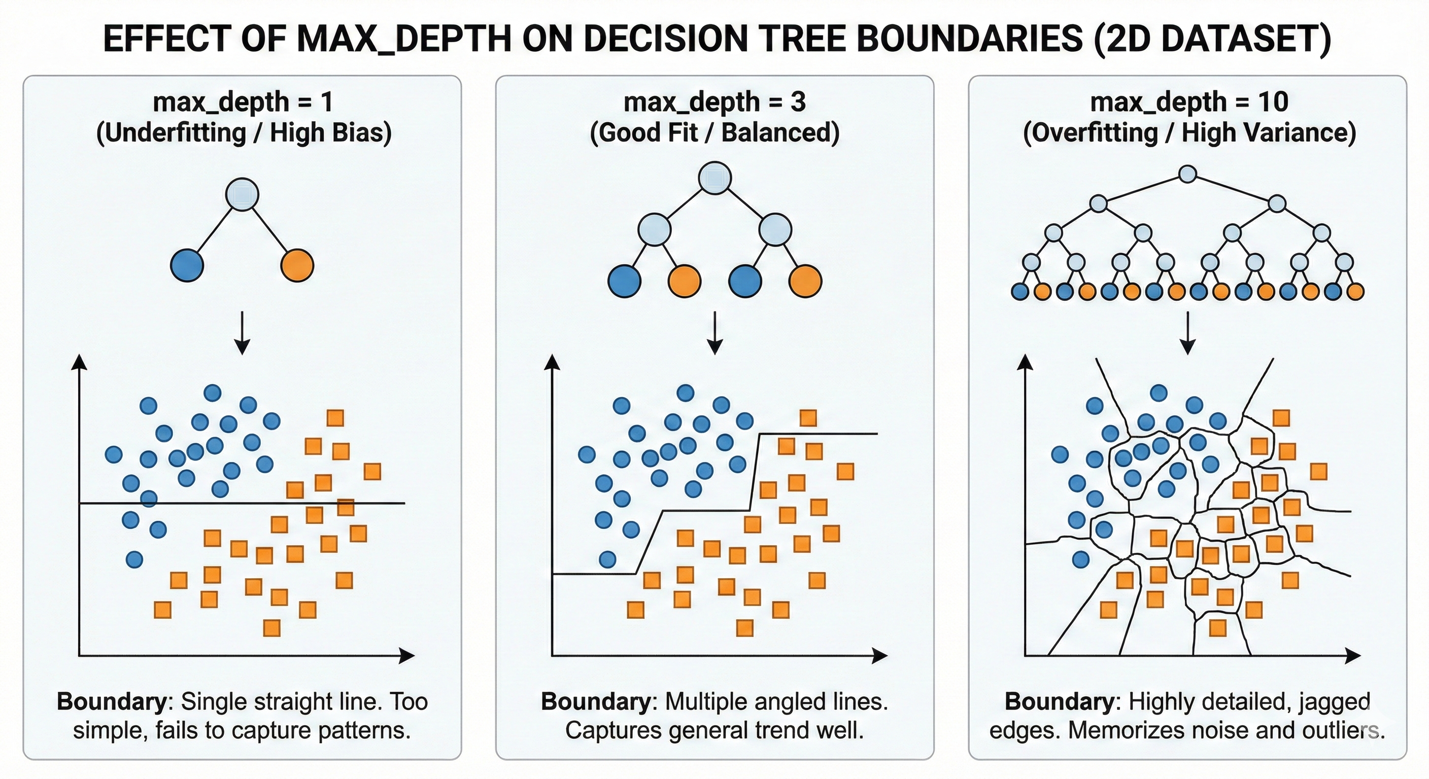
Figure 18. Greater depth leads to more complex decision boundaries and easier overfitting.
min_samples_split (Minimum Samples to Split)
This is the rule: "There must be enough people before I split the group". For example, if a group has only 3 data points and you set min_samples_split = 5, the tree will stop and not split further.
- Low value (2-5): Tree splits very finely → Prone to Overfitting.
- High value (50-100): Tree stops early, roughly → Prone to Underfitting.
min_samples_leaf (Minimum Samples at Leaf)
This rule protects the tips of the tree: "Each leaf after splitting must contain at least how many data points". If a split creates a "lonely" leaf with only 1 data point, that split will be forbidden.
This is extremely important to prevent the model from "memorizing" noise data points (outliers).
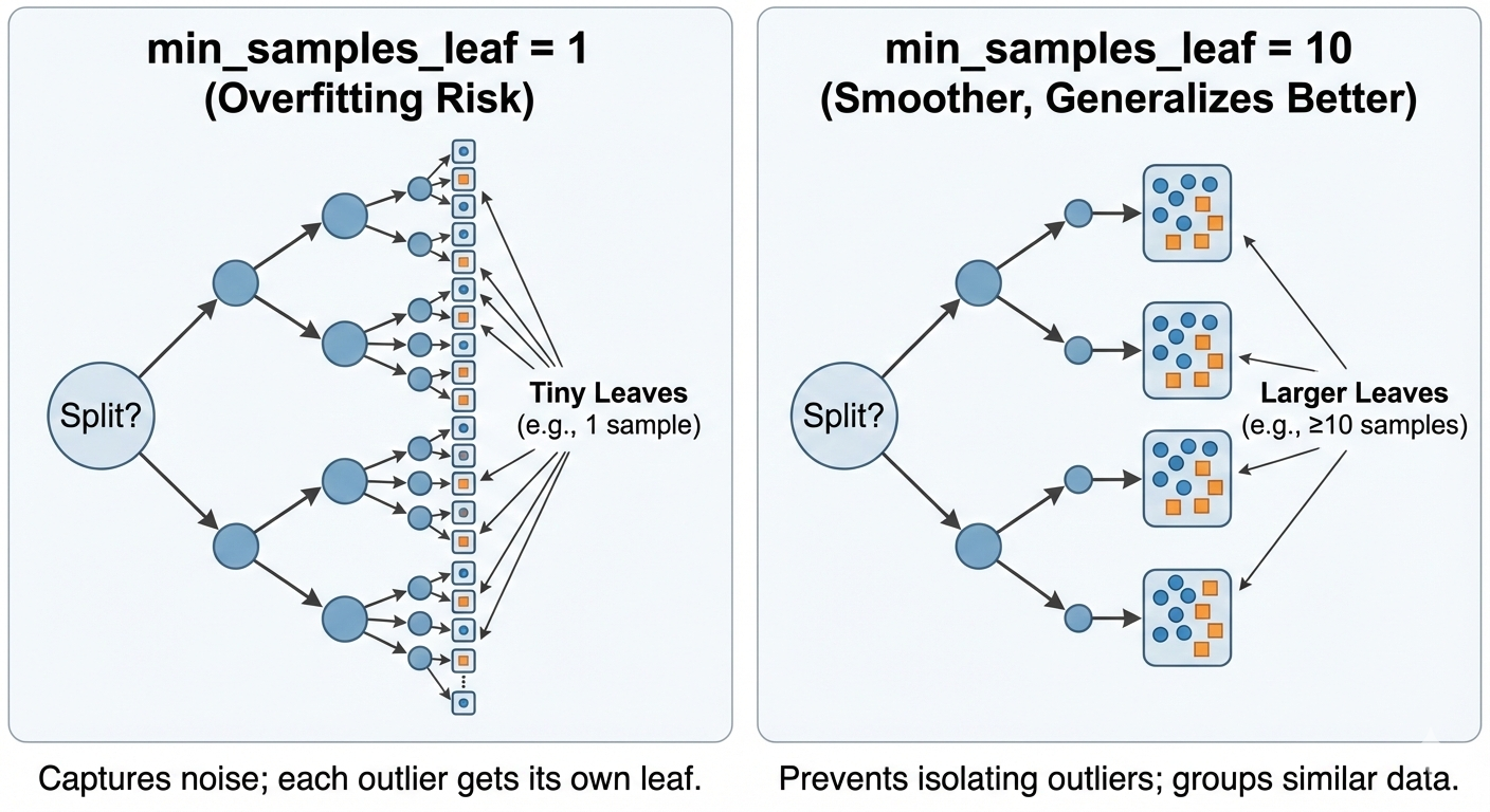
Figure 19. High min_samples_leaf parameter limits the creation of small decision regions.
3.3 Feature Engineering for Decision Tree
One of the reasons Decision Tree is loved is because it's quite "easy-going" with input data.
- No need for Normalization: Trees only care about the order of magnitude to cut (e.g., $x > 5$), so whether data is in the range [0, 1] or [0, 1000] doesn't affect the tree structure.
- Handles both numerical and categorical well: It works with both numerical and categorical features.
However, it has 2 fatal weaknesses that need Feature Engineering to compensate:
3.3.1. Cannot Extrapolate
If your training data only has house prices from 1 billion to 5 billion, Tree will never be able to predict a 10 billion house. Because the nature of Tree is to cut space into regions and assign each region a fixed average value. Outside the learned region, it only knows how to repeat the value of the nearest region.
Solution: Use features that represent change or difference (difference features) instead of absolute values.
3.3.2. Poor at Learning Cross Relationships (Interaction)
Suppose the true pattern is y = x₁ × x₂ (area = length × width). Decision Tree can only cut perpendicularly, so it has to create zigzag stair patterns to approximate the curve of this multiplication, consuming many nodes.
Solution: Help it by pre-creating feature x₃ = x₁ × x₂. Now Tree only needs exactly 1 cut and it's done.
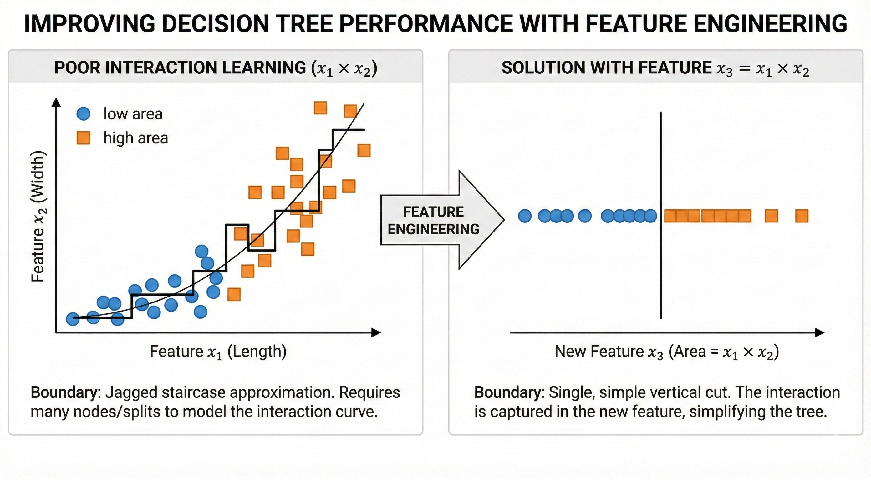
Figure 20. Feature Engineering helps trees recognize complex patterns more easily.
3.4 Validation for Decision Tree
Decision Tree has a bad trait of high Variance. This means that just changing the training data a tiny bit, the tree structure can change completely differently. This makes evaluating the model with a single train/test split unreliable - you might "get lucky" with a good split, or "unlucky" with a bad split.
To overcome this, we use K-Fold Cross-Validation.
Instead of splitting once, we divide the data into $K$ parts (e.g., 5 parts). We take turns using 4 parts to learn and 1 part to test, repeating 5 times like this. The final result is the average of 5 tests. This method helps evaluate more stably and objectively.
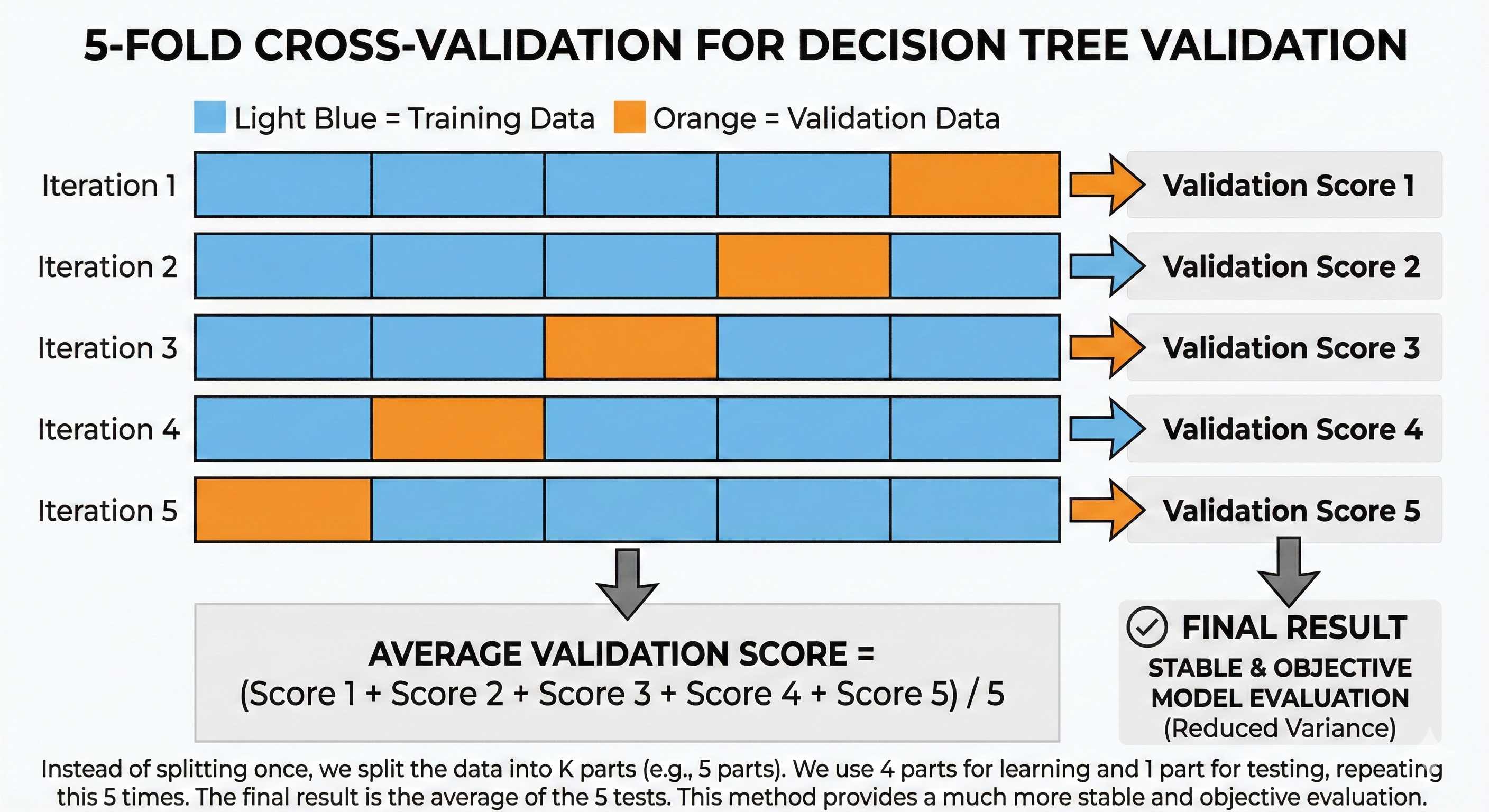
Figure 21. K-Fold Cross-Validation helps evaluate models more stably and objectively.
3.5 Overfitting in Decision Tree
Decision Tree is like a student with super memory but lacking the ability to synthesize thinking. If no one stops it, it will memorize every dot and comma in the textbook (Training data), including printing errors (Noise).
The consequence is that during the semester exam (Validation), encountering new questions without those printing errors, it will get them wrong. This is Overfitting.
Signs: Accuracy on the Train set is nearly perfect (100%), but on the Validation set it's terribly low. The tree grows very deep and has sprawling leaves.
To "restrain" this rote learning, we use Regularization methods, also known as Pruning:
- Pre-pruning: Set rules from the beginning with hyperparameters max_depth, min_samples_leaf... so the tree is not allowed to grow too thick.
- Post-pruning: Let the tree grow freely, then use scissors to cut off excess branches and leaves that don't help with prediction on the validation set.
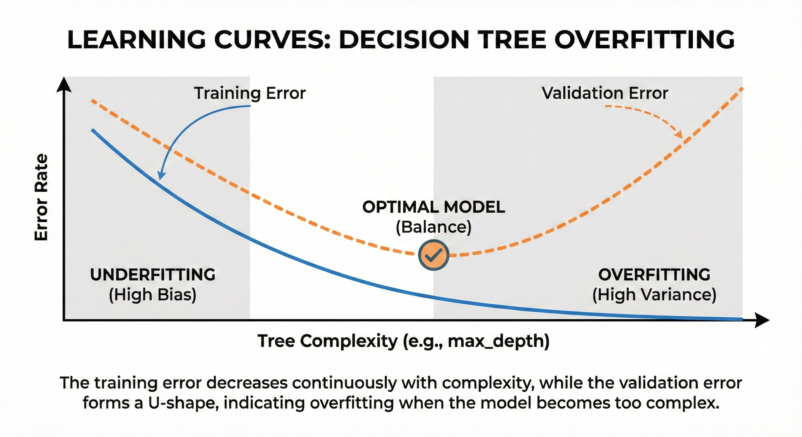
Figure 22. Validation error increases when tree overfits even though training error continues to decrease.
3.6 Bias-Variance in Decision Tree
In summary, a single Decision Tree often falls into a dilemma:
| Depth | Bias | Variance | Condition |
|---|---|---|---|
| Low (1-3) | High | Low | Underfitting |
| High (10+) | Low | High | Overfitting |
It's very difficult for a single tree to achieve both Low Bias and Low Variance at the same time. This is the fatal weakness that led to the birth of Ensemble Learning methods.
Why use one tree when we can plant an entire forest?
- The next section (Random Forest) will use the Bagging strategy to eliminate High Variance.
- The section after that (XGBoost) will use the Boosting strategy to solve High Bias.
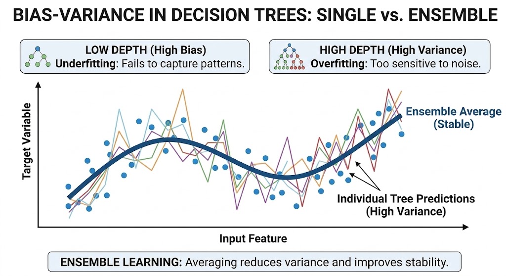
Figure 23. Averaging many trees helps reduce variance and brings stable results.
IV. Random Forest
In the previous section, we saw that a single Decision Tree is like an expert with deep knowledge but very stubborn (high Variance) – just a slight change in data and the opinion changes completely.
So what's the solution? Instead of trusting a single expert, why don't we consult the opinions of an entire council? That's exactly the idea behind Random Forest.
4.1 Introduction to Random Forest
What is Random Forest?
As the name suggests, Random Forest is a "forest" made up of many Decision Trees. However, these are not identical trees. Each tree in the forest is trained on a slightly different version of data and feature set.
The final result of the model is decided by a collective mechanism:
- For Regression problems: Take the average prediction of all trees.
- For Classification problems: Majority Voting – whichever vote gets the most trees wins.
To create this diversity, Random Forest uses two main sources of "randomness":
-
Bootstrap sampling (Bagging): Each tree is trained on a random sample (with replacement) from the original dataset. Statistically, each sample contains about 63% of the original data, the remaining 37% is left out (called Out-of-Bag).
-
Feature randomization: At each split, the tree is not allowed to see all features. It can only randomly select a subset of features to consider (e.g., only 3 out of 10 features). Usually $\sqrt{n}$ for classification and $n/3$ for regression.
Why is "random" good?
Imagine you want to predict tomorrow's weather and ask 100 meteorologists.
-
If all 100 people studied at the same school, use the same software, and read the same weather report, they will give 100 identical answers. If wrong, the whole group is wrong.
-
But if each person uses their own data source, one looks at humidity, one looks at wind direction, one measures temperature... their answers will be very diverse.
In that case, if you take the average opinion of these 100 people, individual errors (some guessing too high, some too low) will cancel each other out. What remains is the most correct signal.
4.2 Hyperparameters of Random Forest
Because Random Forest is a collection of Decision Trees, it inherits all hyperparameters of Tree (like max_depth, min_samples_split). However, it has some additional characteristic "knobs".
n_estimators (Number of Trees)
This is the total number of trees in your forest.
-
Effect: Unlike other models, increasing the number of trees in Random Forest almost never causes Overfitting. The reason is that trees are trained independently, adding trees only makes the averaging calculation smoother and more stable.
-
Tradeoff: More trees means higher accuracy, but training and prediction speed will slow down.
-
Rule of thumb: Usually 100-500 trees is enough. Beyond this threshold, the benefit gained will saturate (diminishing returns) – adding 1000 more trees might only increase accuracy by 0.01% but takes twice as long.
max_features (Number of Features Considered per Split)
This is the most important hyperparameter to control forest diversity. At each split node, the tree is only allowed to randomly select max_features features to evaluate.
-
If set too high (close to total features): Trees will become identical (because every tree chooses the best feature). Diversity decreases → Effectiveness of averaging decreases.
-
If set too low: Trees will be too weak and random, unable to learn any pattern.
-
Recommended level: $\sqrt{n\_features}$ for classification and $n\_features/3$ for regression.
Why are similar trees a problem? Look at the variance formula of Random Forest:
$$Var(RF) = \rho\sigma^2 + \frac{(1-\rho)\sigma^2}{n}$$
Where $\rho$ is the correlation between trees. When max_features is high → trees all choose the same best feature → $\rho$ increases → the $\rho\sigma^2$ part dominates → averaging is no longer effective. Conversely, low max_features forces trees to "be creative" with different features → $\rho$ decreases → overall variance decreases significantly.
max_depth (Maximum Depth)
-
Let trees grow naturally (max_depth = None): This is the default of the Scikit-learn library. Each tree will be very complex with high Variance, but thanks to the forest's averaging mechanism, overall Variance will decrease.
-
Limit depth (max_depth = 10-20): Helps the model be lighter, run faster, and sometimes helps avoid overfitting on small datasets.
4.3 Feature Engineering for Random Forest
Random Forest inherits the "easy-going" nature of Decision Tree:
- No need for data Normalization/Standardization.
- Handles both numerical and categorical data well.
Feature Importance — Secret Weapon
An extremely strong point of Random Forest is the ability to self-evaluate which features are important. It does this by measuring how many times a feature is used to split and how much it helps reduce impurity.
We can use this feature for Feature Selection – removing redundant features to make the model run faster and less noisy.
However, don't forget that Random Forest still has Tree's weakness: Cannot extrapolate. If training data only has values up to 100, it cannot predict the value 200. Therefore, feature engineering techniques creating differences or ratios are still very necessary.
4.4 Validation for Random Forest
Random Forest has a "free" and extremely powerful validation mechanism called Out-of-Bag (OOB) Error.
Remember that each tree is trained on only about 63% of the data (Bootstrap sample). So where does the remaining 37% go? They are called Out-of-Bag (OOB) samples – samples that the tree has never seen.
Instead of having to cut a separate Validation set, we can use these OOB samples themselves to test each tree's ability.
-
Mechanism: For each data point $X$, we only take predictions from trees that don't contain $X$ in their training set. The average error of these predictions is the OOB Error.
-
Benefit: Maximizes data utilization for training, especially valuable when you have little data.
However, you should still use traditional Cross-Validation when:
- Need to compare Random Forest with other algorithms (like SVM, Linear Regression).
- Tuning hyperparameters (OOB score is sometimes too optimistic).
- Working with Time Series data – because OOB doesn't respect time order.
4.5 Overfitting in Random Forest
Why does RF Overfit less than a single tree?
The secret lies in mathematics: If you have $n$ independent random variables all with variance $\sigma^2$, then the variance of their average will decrease to $\sigma^2/n$.
However, in practice trees are not completely independent because they learn from the same data source. The more accurate formula is:
$$Var(RF) = \rho\sigma^2 + \frac{(1-\rho)\sigma^2}{n}$$
Where $\rho$ is the average correlation between trees.
This explains why max_features is important: low max_features → reduces $\rho$ (trees are less similar) → averaging is more effective → Variance decreases more strongly.
When can RF still Overfit?
Although very robust, Random Forest is not immortal. It can still "rote learn" when:
- Too little data: Makes bootstrap samples too similar, losing diversity.
- Too noisy data: If features contain too much garbage, all trees will learn that garbage together.
- max_features too high: Makes trees become too similar (High Correlation).
4.6 Bias-Variance in Random Forest
This is how Random Forest solves the Bias-Variance tradeoff:
- Bias: It maintains the low Bias level of decision trees (by allowing deep trees).
- Variance: It strongly reduces Variance by averaging many trees.
The result is that we have a Low Bias, Low Variance model – the dream of every Data Scientist.
However, there's a small issue: Random Forest is only good at reducing Variance (fluctuation). If the component trees themselves all "aim wrong" (High Bias) – for example, all missing some complex pattern – then averaging also can't help them aim more accurately.
So how to reduce Bias too? How to make trees not only learn independently but also know how to "correct each other"? That's the story of Boosting and the masterpiece XGBoost that we'll explore in the next section.
V. XGBoost
Although the "crowd strategy" (Bagging) helps Random Forest minimize fluctuation (Variance) extremely well, it's helpless when council members all make the same mistakes. If the trees themselves all have high Bias – meaning they all miss some complex pattern in the data – then averaging also can't turn wrong into right.
To solve this problem, we can no longer just rely on "overwhelming with numbers". We need a more sophisticated strategy: instead of training in parallel independently, train sequentially. The successor is born to correct the predecessor's errors. That's the core thinking of Boosting, and the pinnacle of this school is XGBoost.
5.1 Introduction to XGBoost
To understand how XGBoost operates, imagine you're standing on top of a foggy mountain and the task is to get down to the lowest valley (where error is lowest) as fast as possible. Because the fog is thick, you can't see the destination. The wisest strategy at this moment is to look right at your feet, feel which direction is steepest downward and take a step in that direction. After each step, you stop again to observe the new slope and continue.
In Machine Learning, this "path-finding" method following the slope is called Gradient Descent. XGBoost (Extreme Gradient Boosting) applies exactly this thinking: each tree generated is a "step" leading the model to where there's lower error.
Technically, XGBoost builds trees sequentially. The first tree learns on the original data. Then, we calculate errors (Residuals) – the difference between actual and predicted values. The second tree is generated not to predict the original value anymore, but to predict that error itself. This process repeats continuously, with later trees always trying to compensate for earlier trees' shortcomings.
The core difference lies in: If Random Forest uses deep and complex trees to reduce Variance, then XGBoost uses very shallow and simple trees (Shallow trees/Weak learners) to gradually reduce Bias.
5.2 Hyperparameters
XGBoost's power comes with complexity. To control this "racing car", you need to master the following important control knobs:
learning_rate ($\eta$ - eta)
Back to the mountain descent example, learning_rate is your stride length. If your stride is too long ($\eta$ high, e.g., 0.3), you descend very fast but easily slip, step too far past the lowest point and climb up the other slope. Conversely, if your step is too short ($\eta$ low, e.g., 0.01), you walk very safely and accurately, but it will take an extremely long time (need many trees) to reach the destination. This is the tradeoff between convergence speed and optimal accuracy.
Technically, each new tree contributes to the prediction according to the formula:
$$\hat{y}_{new} = \hat{y}_{old} + \eta \times prediction_{tree}$$
With $\eta$ = 0.1, the new tree can only "contribute" 10% to the final result. This has 2 benefits:
- If the new tree predicts wrong, the error only affects 10% instead of 100%
- Allows later trees to "fine-tune" gradually instead of changing suddenly
n_estimators (Number of Trees)
Unlike Random Forest where "the more the merrier", the number of trees in XGBoost is a double-edged sword. Because each tree is born to correct errors, if you allow too many trees to train, at some point the model will run out of "real" errors to fix and start "fixing" random noise too. This leads straight to Overfitting. Therefore, in XGBoost, we rarely choose a fixed n_estimators number but usually let it automatically stop using the Early Stopping technique.
max_depth (Maximum Depth)
In XGBoost, we usually use very shallow trees, depth only about 3-7 (very different from RF which is often very deep). The reason is that Boosting's philosophy is combining many "weak learners". Each tree only needs to solve a small part of the problem (a simple pattern). Trying to force a tree to learn too deep from the start will break this sequential error-correction strategy.
gamma ($\gamma$ - min_split_loss)
This is an important hyperparameter controlling whether a node is allowed to split or not. Specifically, gamma specifies the minimum loss reduction required for a split to be accepted.
- gamma = 0: All splits are allowed, as long as they reduce loss (even by just 0.0001).
- gamma high (e.g., 1-5): Only splits that create significant improvement are performed → simpler tree, less overfitting.
In other words, gamma acts as a "filter" preventing the tree from creating trivial branches with no real value.
Other Anti-Overfitting Parameters
To minimize rote learning risk, XGBoost integrates a series of defense mechanisms:
subsample & colsample_bytree: Borrowing ideas from Random Forest, each tree only sees a random portion of data and features.
Why is randomization needed in XGBoost? Unlike Random Forest (independent trees), in XGBoost trees depend on each other — later trees learn from earlier trees' errors. If every tree sees 100% of data, they will all be "obsessed" by the same outliers or noise. subsample=0.8 means each tree only sees 80% random rows. An outlier appearing in this tree may be "hidden" from that tree → the overall model is less sensitive to noise.
reg_alpha (L1) & reg_lambda (L2): This is what makes the "Extreme" in the name. It integrates Regularization components directly into the loss function to penalize overly complex models.
L2 Regularization (reg_lambda) works like a "tax" on the magnitude of weights at leaves. XGBoost's objective formula has the form:
$$Loss = \sum(errors) + \lambda \times \sum(w^2)$$
Where $w$ is the prediction value at each leaf. When $\lambda$ increases:
- The model is "penalized" for making predictions that are too extreme ($w$ too large)
- Forces leaves to be more "modest" → reduces overfitting
Example: If 1 leaf contains only 2 data points and both have value = 100, a model without regularization will predict $w$ = 100. But with high $\lambda$, it will predict $w$ = 80 (lower) because "not enough evidence to be that confident".
5.3 Feature Engineering and Data Processing
XGBoost is smarter than traditional tree models in its ability to automatically handle Missing Values. When encountering missing values (NaN), it doesn't throw an error but will learn: "For this feature, if data is missing, should we go to the left or right branch to reduce error best?". Therefore, you have less burden of having to manually impute data.
For Feature Importance, XGBoost provides a much more multi-dimensional view. You can evaluate the importance of a feature based on Gain (how much error reduction it provides - most important for accuracy), Cover (data coverage), or Weight (frequency of appearance in trees). Depending on the purpose of the problem, you choose the appropriate measure.
5.4 Validation and Early Stopping
Because XGBoost easily Overfits if trained too long, the Early Stopping technique is almost mandatory in practice. The process is very simple: we set aside a portion of data as a Validation set. After each iteration (when a new tree is generated), we immediately check the error on this set. If the error doesn't decrease for a number of consecutive rounds (e.g., 10 rounds), we immediately stop training and take the model at the best time before that.
5.5 Overfitting in XGBoost
Why is XGBoost more prone to Overfitting than Random Forest? Imagine training XGBoost is like a perfectionist student doing homework.
- Early stage: The student corrects large formula errors (this is learning real knowledge).
- Later stage: When there are no more large errors, they start scrutinizing trivial details like ink smudges or the slant of handwriting and try to "fix" them thinking they're errors.
- Consequence: The work becomes mechanical, unnatural, and can't be applied to other tests.
In XGBoost, "ink smudges" are Noise. If we let the model correct errors too long, it will memorize noise too. To prevent this, we need to build multiple layers of defense (Defense in Depth):
- Control complexity: Use shallow trees (low max_depth) and set
gamma> 0 so the model can't learn overly trivial details. - Randomization: Use subsample and colsample_bytree (like Random Forest) so each tree only sees part of the data, avoiding being obsessed by local noise.
- Penalization (Regularization): Increase reg_alpha (L1) and reg_lambda (L2) to force the model's weights to simplify.
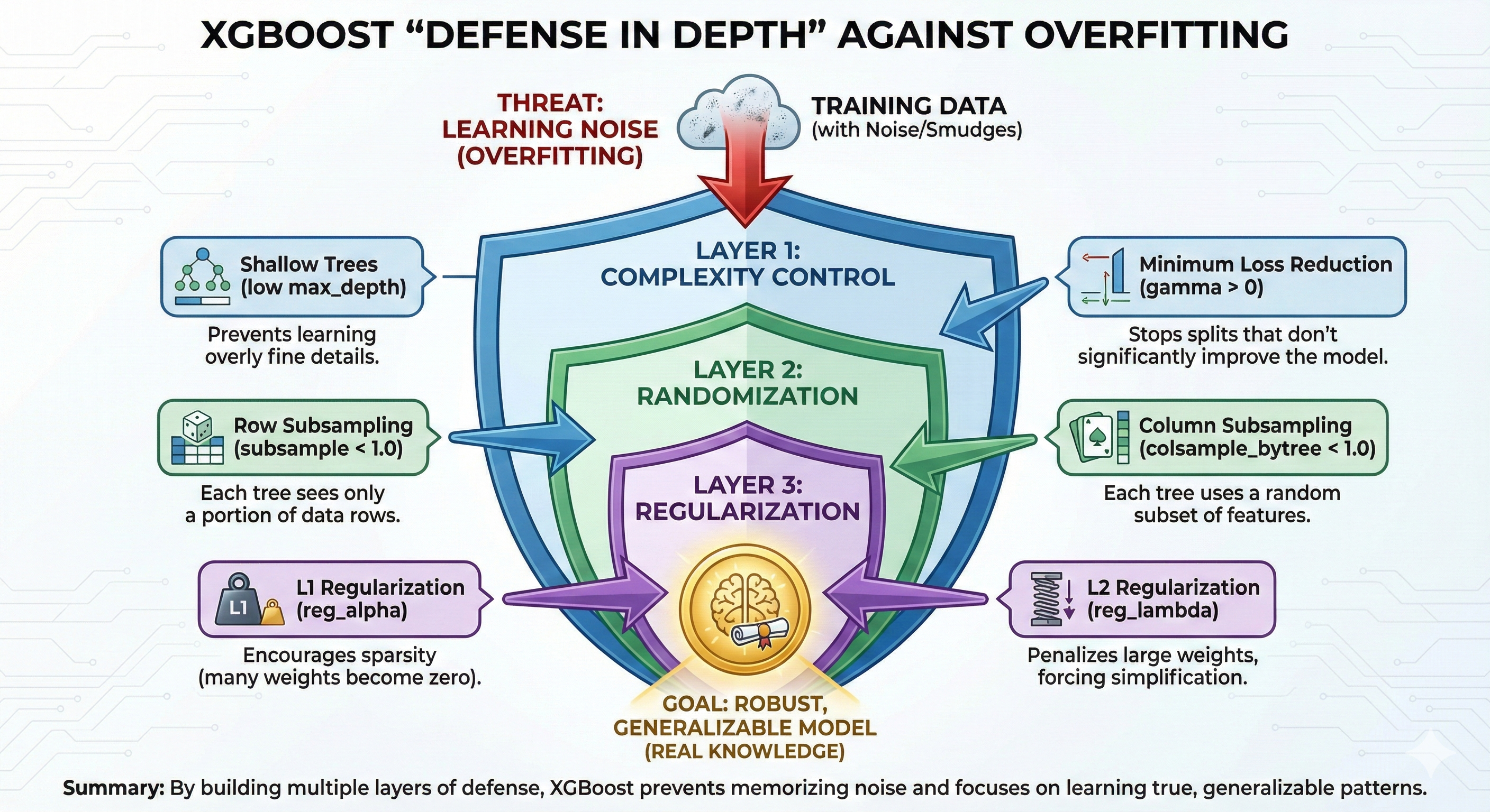
Figure 24. XGBoost's mechanisms help effectively control Overfitting.
5.6 Bias-Variance in XGBoost
Finally, let's look at XGBoost's position in the overall picture of Bias-Variance balance, comparing directly with its sibling Random Forest:
| Aspect | Random Forest | XGBoost |
|---|---|---|
| Components | Deep trees (Low Bias, High Variance) | Shallow trees (High Bias, Low Variance) |
| Mechanism | Averaging | Sequential Correction |
| Main effect | Strongly reduce Variance | Strongly reduce Bias |
Bias reduction mechanism:
XGBoost starts with a very naive tree (high Bias). But through hundreds of consecutive corrections, Bias is gradually polished down to nearly 0. This is why XGBoost usually achieves higher accuracy than Random Forest on complex datasets.
Sweet Spot:
However, the price to pay is that when Bias decreases deeply, Variance tends to increase (model becomes sensitive). The art of using XGBoost is finding the right stopping point – where Bias is low enough (accurate enough) but Variance hasn't increased too high yet. And the most powerful tool to find that point is Early Stopping that we discussed in section 5.4.
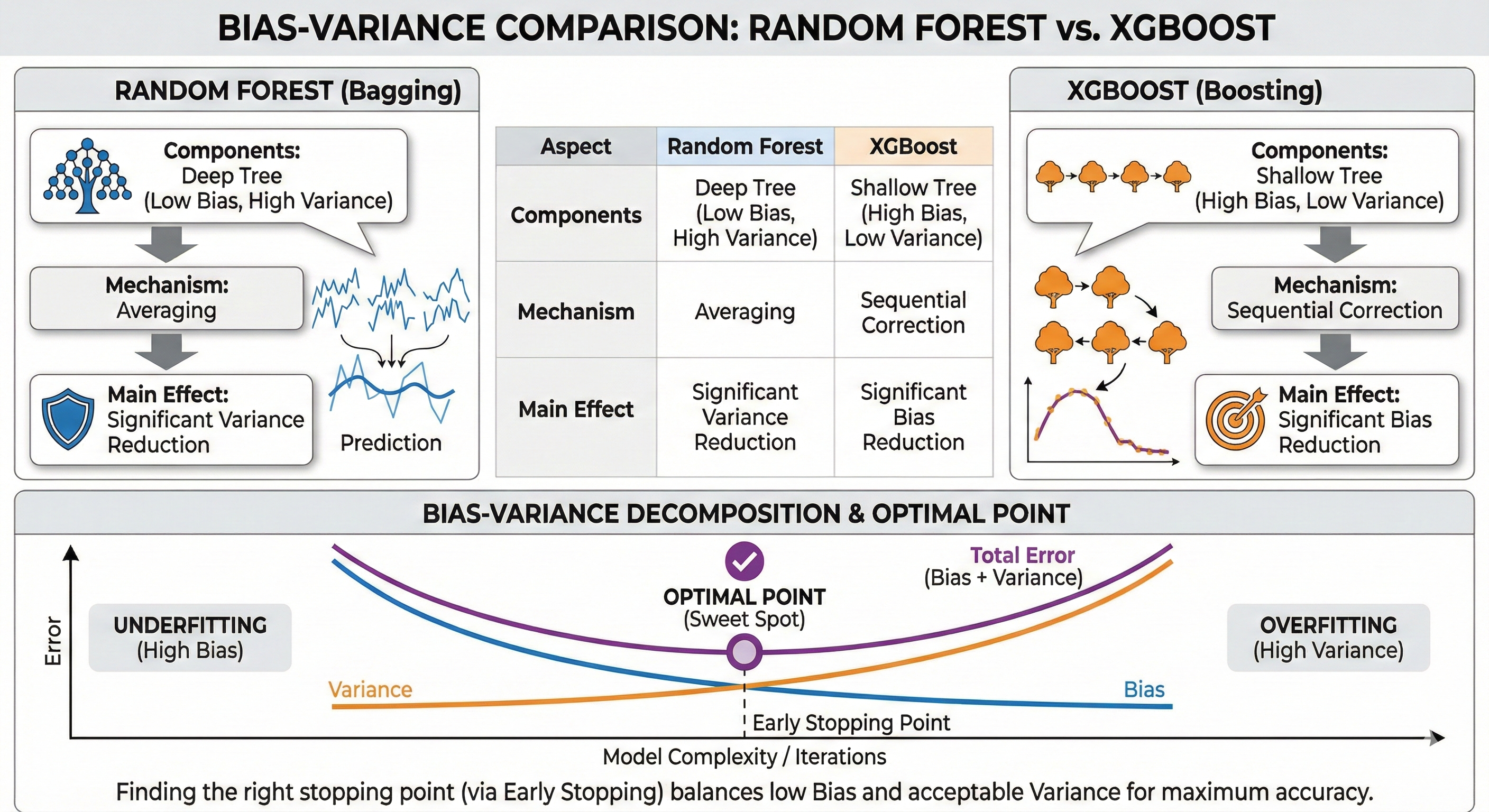
Figure 25. The balance between Bias and Variance at the U-shaped bottom optimal point.
VI. Specifics for Time Series Data
If Random Forest or XGBoost are powerful "warhorses", then Time Series data is a "racecourse" with extremely treacherous terrain. If you bring the mindset of regular data here, you're likely to have an accident at the first turn.
Why? Because in Time Series, time is king.
6.1 Why is Time Series Special?
Core characteristics:
In regular problems (like image recognition or customer classification), the position of data rows doesn't matter. You can shuffle them freely. But with Time Series, order is inviolable. An observation at time $t$ always depends closely on what happened before ($t-1, t-2...$).
Problem with regular methods:
Imagine you're attending a stock price prediction class. While studying for the exam, the teacher accidentally shows you tomorrow's price answer in advance. Of course, you'll do extremely well on the exam. But when investing in reality, you no longer have that answer sheet, and you lose heavily.
In Machine Learning, this phenomenon is called Data Leakage.
If you use regular K-Fold Cross-Validation (which shuffles data randomly) for Time Series, you're inadvertently putting "future" information (e.g., March) into the training set to predict "past" (e.g., February). The evaluation results will be illusory high and meaningless.
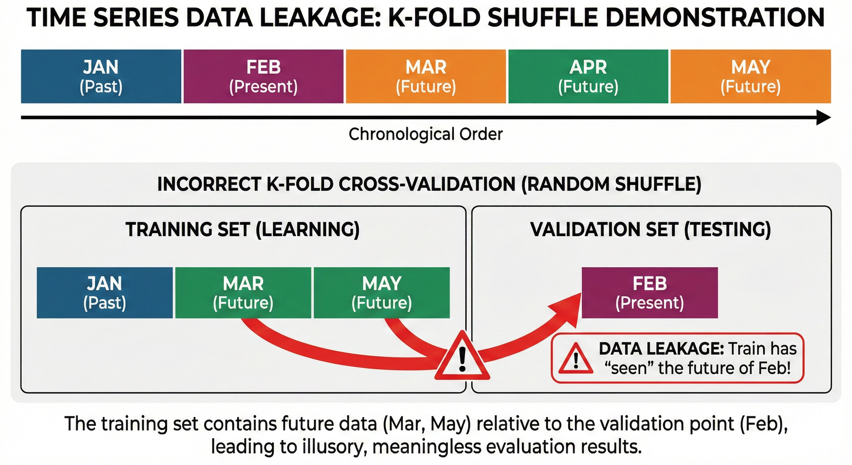
Figure 26. K-Fold shuffle causes future data leakage into the training set.
6.2 Types of Features for Time Series
Models like XGBoost or Random Forest don't inherently understand concepts like "yesterday" or "last week". We must teach them through Feature Engineering.
Lag Features
This is the simplest way to tell the model about the past.
- Definition: The value of a variable at previous time points.
- Example:
price_lag_1is yesterday's price,price_lag_7is last week's price. - Meaning: Captures Autocorrelation. Today's price usually has a close relationship with yesterday's price. Choosing which lag depends on domain knowledge: for daily data, lags 1, 7, 30 are usually important; for hourly data, lags 1, 24, 168 (1 week).
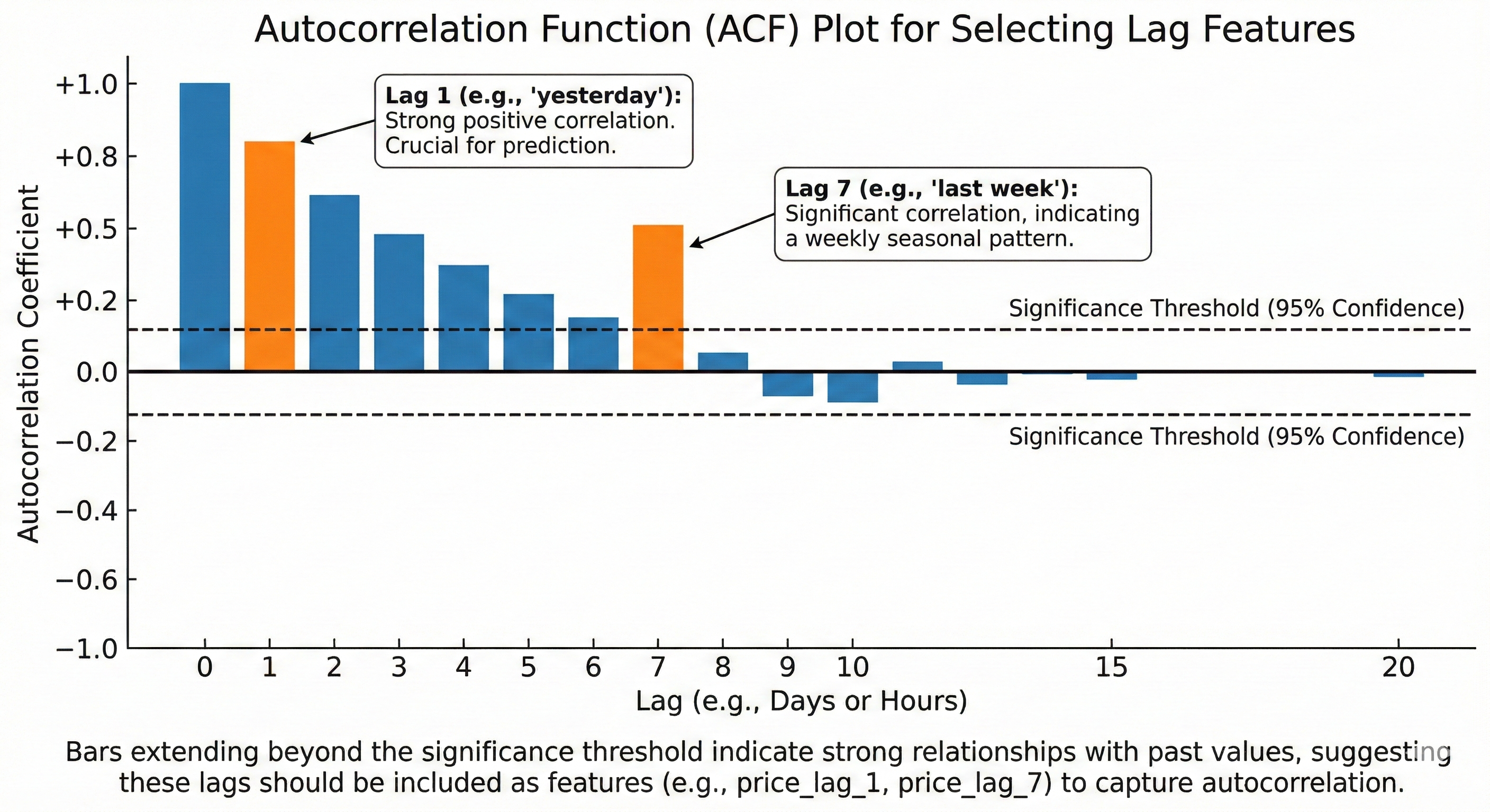
Figure 27. ACF chart supports finding lags with high correlation.
Rolling/Window Features
Instead of just looking at a single past point, we look at a time period (window) to summarize the trend.
Common types:
- Rolling mean: Average price of the last 7 days (represents trend).
- Rolling std: Standard deviation of the last 7 days (represents volatility).
- Rolling min/max: Bottom and peak in 7 days.
Choosing Window size: Small windows (5-10) help the model be sensitive to fast changes but prone to noise. Large windows (20-50) give smoother signals but react slowly to the market.
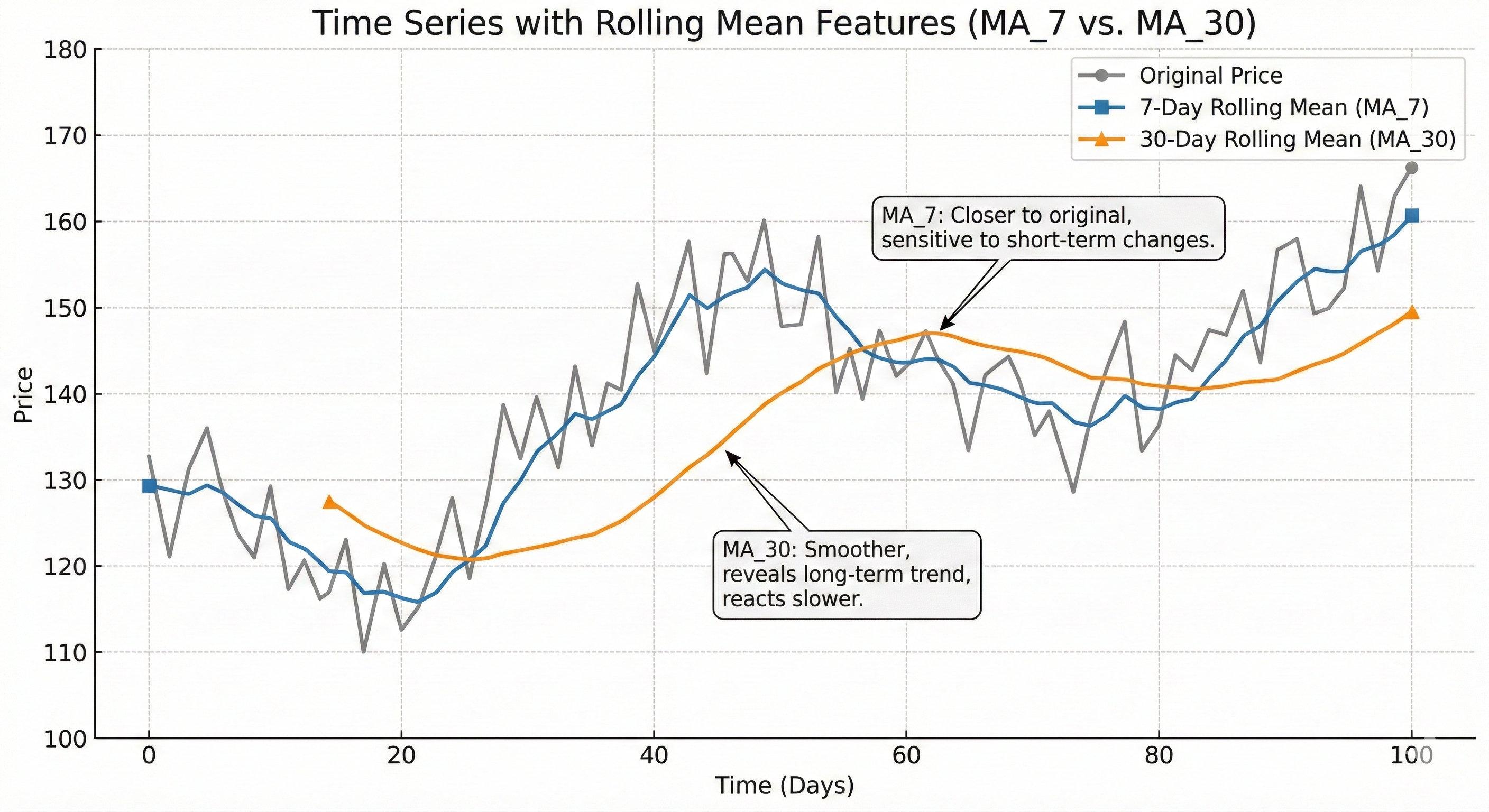
Figure 28. Rolling mean with different windows helps capture multiple timeframes.
Difference Features
If you remember Blog 1 about Derivatives, then Difference is the discrete version of derivatives.
- Formula:
diff_1 = price(t) - price(t-1). - Meaning: Helps remove trend to bring data to a stable form (stationary). Instead of making the model predict Bitcoin price is $50,000 (a very large absolute number that changes constantly), make it predict whether today's price increased or decreased by how much compared to yesterday. This is much easier to learn.
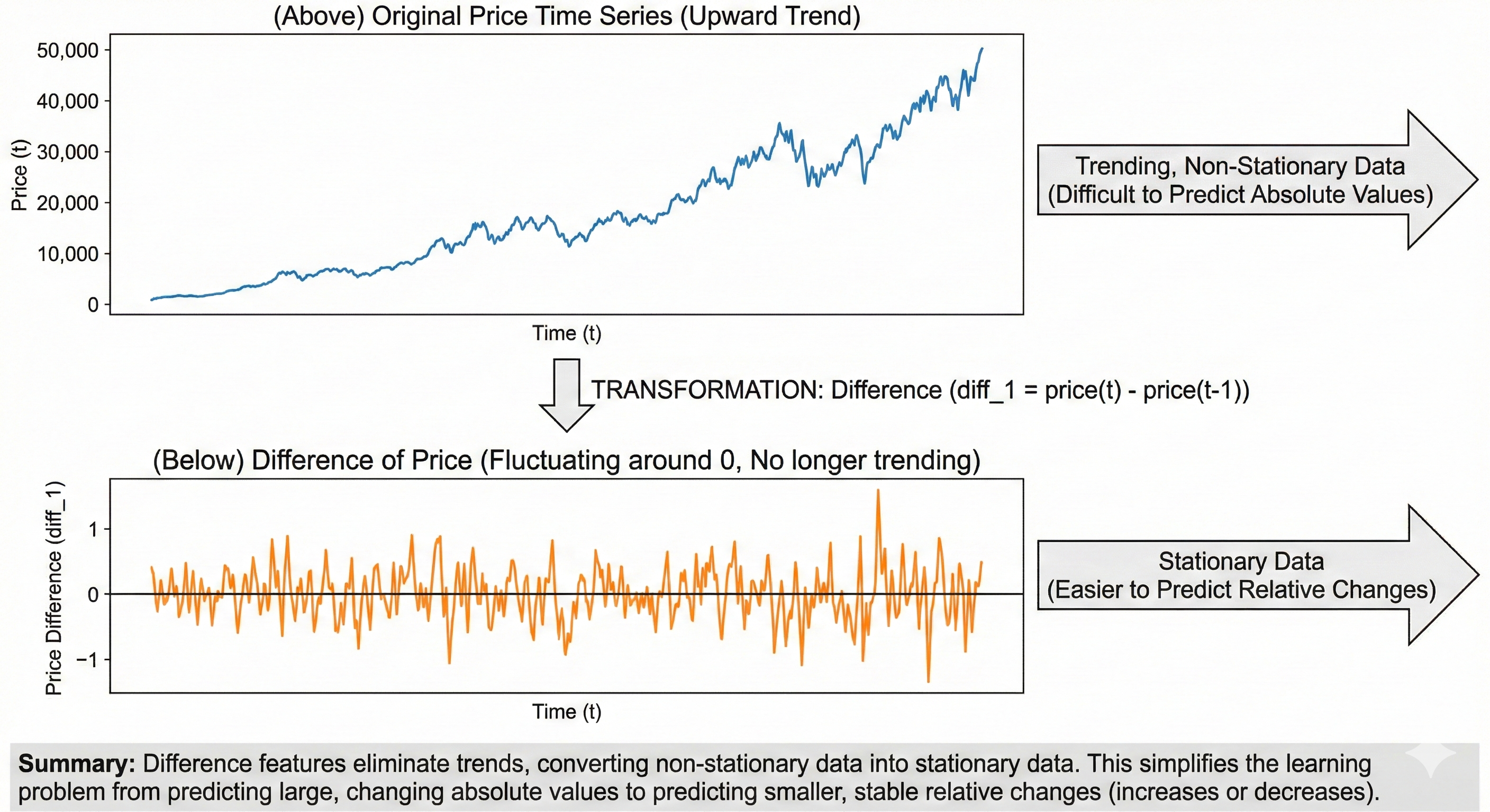
Figure 29. Differencing handles trend, helping the model focus on patterns.
Calendar/Seasonal Features
Time has cyclical nature: 11 PM and 12 AM are actually very close (only 1 hour apart), but numerically (23 vs 0) they're very far. If you put numbers 0-23 directly into the model, it will misunderstand.
Solution: Use Cyclical encoding with Sin and Cos functions.
hour_sin = sin(2π × hour / 24)hour_cos = cos(2π × hour / 24)
This method transforms time onto a trigonometric circle, preserving its cyclical nature.
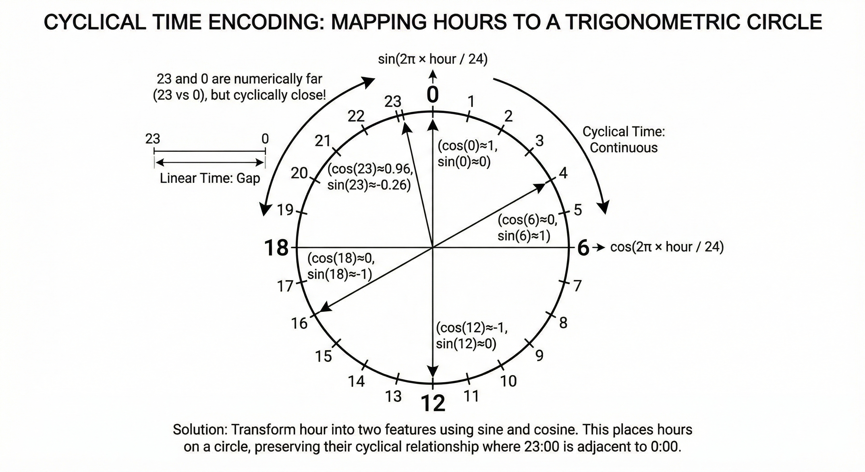
Figure 30. Cyclical encoding helps maintain time continuity.
Critical Note: Avoid Data Leakage
When creating features, be extremely careful. At time $t$, you are only allowed to use data up to $t-1$.
- Wrong: Calculate average from day $t-6$ to day $t$ (already leaked day $t$!).
- Correct: Calculate average from day $t-7$ to day $t-1$.
6.3 Validation for Time Series
Since regular K-Fold is forbidden, we need validation strategies that respect the flow of time.
Walk-Forward Validation
The idea is to always train on the past and validate on the near future, like learning through grade 1 then testing grade 1, learning through grade 2 then testing grade 2.
- Split 1: Train [Jan-Mar], Validate [Apr]
- Split 2: Train [Jan-Jun], Validate [Jul]
- Split 3: Train [Jan-Sep], Validate [Oct]
This method simulates reality exactly: "I have data up to yesterday, I need to predict today".
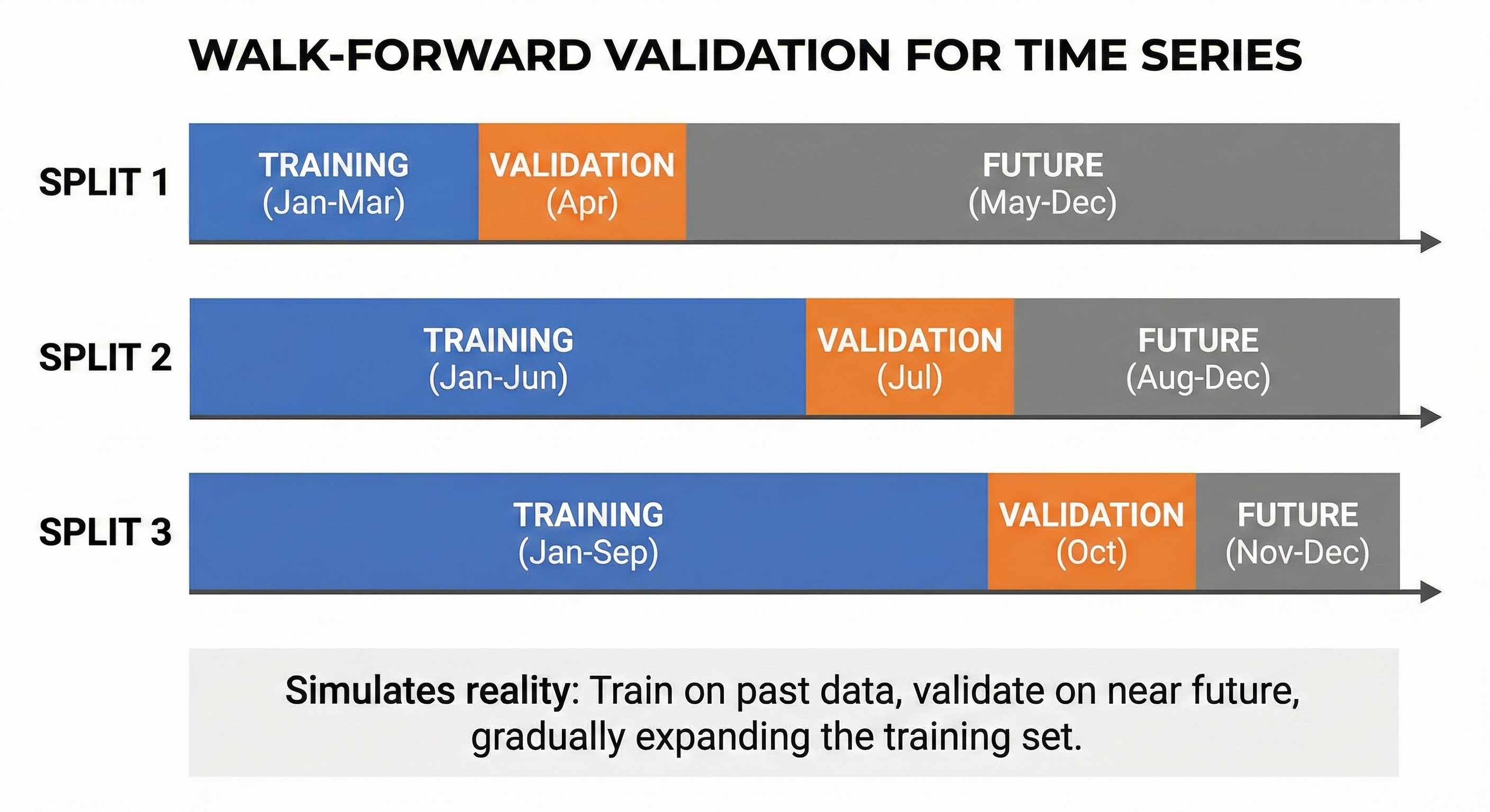
Figure 31. Walk-Forward Validation maintains time sequence during validation.
Sliding Window Validation
Unlike Walk-Forward (the more you learn, the more you remember), Sliding Window has limited memory. The training window has a fixed size and slides forward over time.
This method is suitable when you believe data that's too old no longer has value, or market patterns have changed (concept drift).
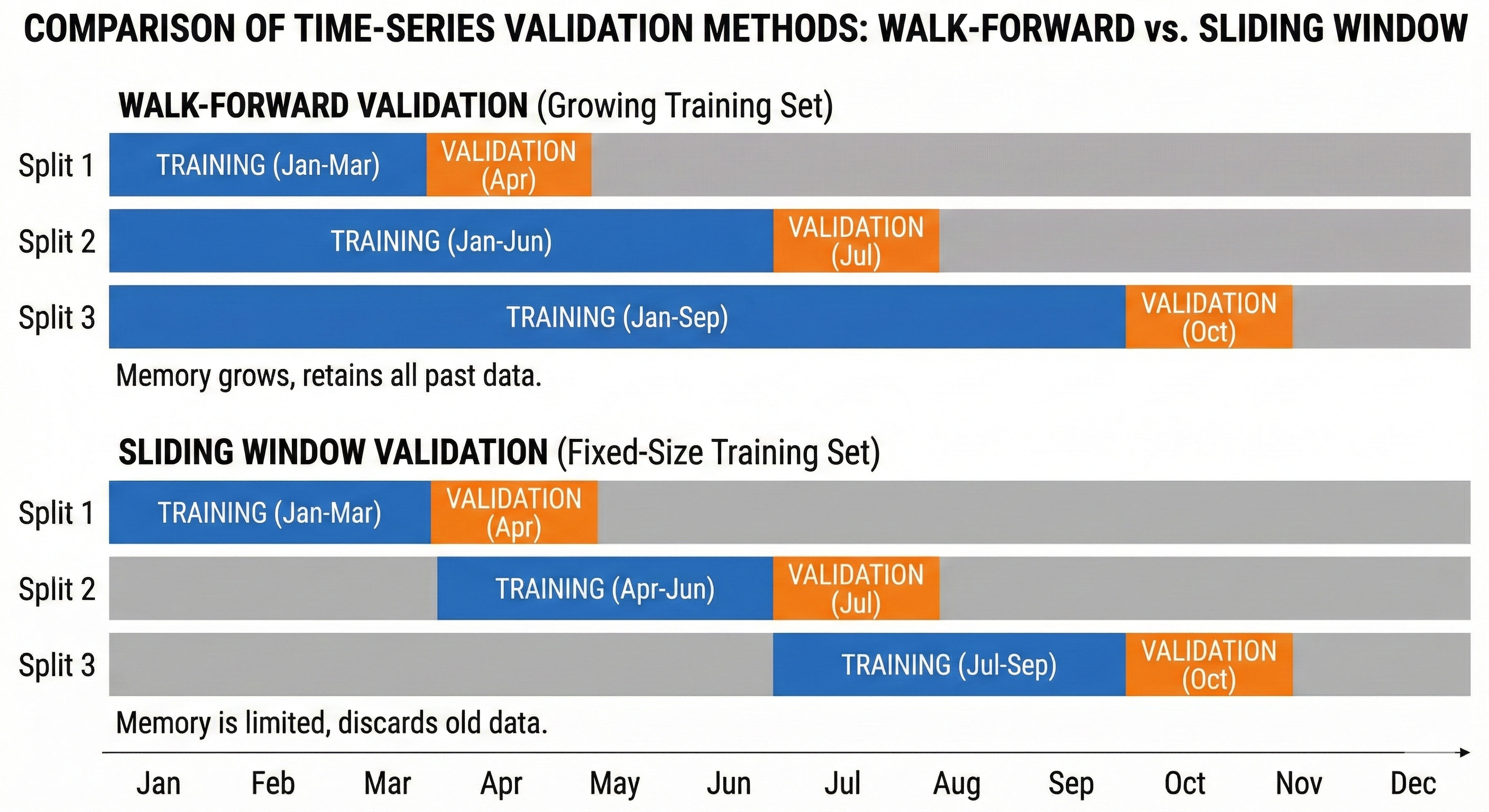
Figure 32. Expanding Window keeps history, Sliding Window keeps only recent data.
Purging and Embargoing — Advanced Techniques
Even when splitting correctly by time, leakage can still occur due to overlapping features.
Example: You use rolling_mean_7 (7-day average). If the last day of the Train set is day 30, its feature contains information from days 24-30. The first day of the Validation set is day 1, its feature contains information from days 25-31.
Clearly, information from days 25-30 is appearing in both sets!
Solution (Purging): Leave a gap between Train and Validation sets. The size of this gap must be larger than the largest lag of features to cut off the dependency.
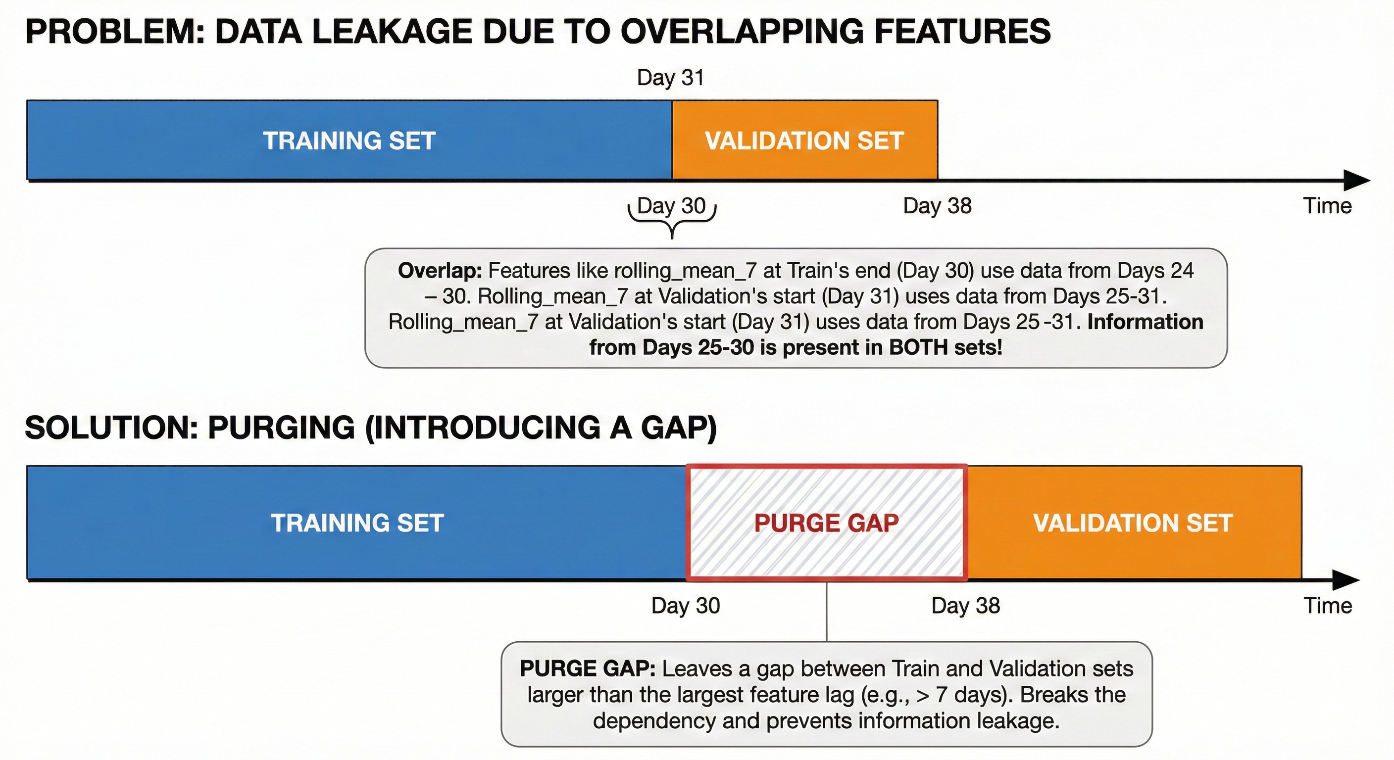
Figure 33. Purge Gap limits overlap between lag features.
VII. Practice — Hyperparameter Configuration
We've come a long way: from understanding model essence (Decision Tree, RF, XGBoost) to handling specific data (Time Series). But having good data and fancy models is only a necessary condition. For the machine to actually run smoothly and achieve the highest performance, you need to know how to turn the "adjustment knobs" — also known as Hyperparameters.
Leaving default values usually gives only average results. Below are baseline configurations distilled from practice, helping you save time fumbling around.
7.1 Basic Configuration for Decision Tree
Decision Tree is the simplest model, but also the easiest to "rote learn" (overfit) if not controlled.
Declaration form (Python sklearn):
from sklearn.tree import DecisionTreeRegressor # or DecisionTreeClassifier

model = DecisionTreeRegressor(
    max_depth=5,              # Maximum depth: the most important checkpoint
    min_samples_split=10,     # Need at least 10 samples to continue splitting
    min_samples_leaf=5,       # Each leaf must have at least 5 samples (avoid lonely leaves)
    random_state=42           # For reproducibility
)
Baseline values table:
| Hyperparameter | Baseline Value | Common Range | Notes |
|---|---|---|---|
| max_depth | 5 | 3 - 15 | If set to None, tree will grow until leaves are pure (very easy to overfit). |
| min_samples_split | 10 | 2 - 50 | Higher value → less detailed tree → less overfit. |
| min_samples_leaf | 5 | 1 - 20 | More important than split. Prevents creating groups that are too small. |
Tips from practice:
- Start with
max_depth = Noneto see how complex the tree can get, then gradually tighten (max_depth = 10, 5...). - In practice,
min_samples_leafis usually more effective at fighting noise thanmin_samples_split.
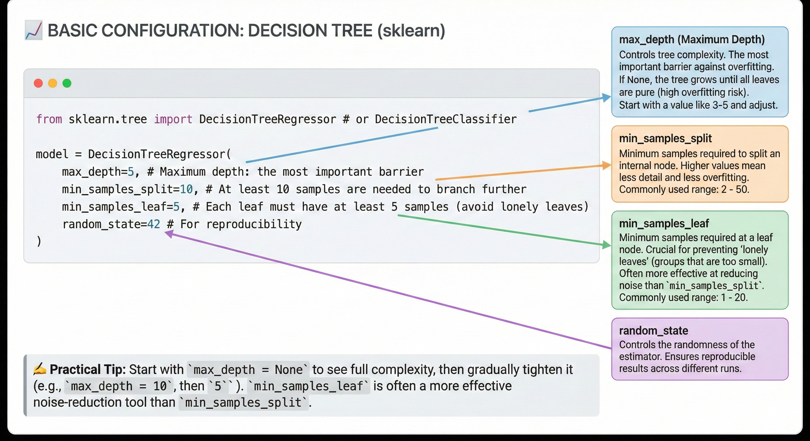
Figure 34. Basic Decision Tree configuration and parameter meanings.
7.2 Basic Configuration for Random Forest
Random Forest is much more "benign". Thanks to the averaging mechanism, it's harder to overfit than a single tree, so you can be more relaxed with complexity parameters.
Declaration form (Python sklearn):
from sklearn.ensemble import RandomForestRegressor # or RandomForestClassifier

model = RandomForestRegressor(
    n_estimators=200,         # Number of trees in the forest
    max_depth=None,           # Let trees grow naturally (RF handles variance well so no fear)
    max_features='sqrt',      # Number of random features at each split
    min_samples_leaf=1,       # Default
    n_jobs=-1,                # Use all CPU cores to run in parallel (important!)
    random_state=42,
    oob_score=True            # Utilize OOB for free validation
)
Baseline values table:
| Hyperparameter | Baseline Value | Common Range | Notes |
|---|---|---|---|
| n_estimators | 200 | 100 - 500 | More trees rarely decreases accuracy, only costs RAM/CPU. |
| max_depth | None | None or 10-30 | None is the most common choice because RF self-reduces variance. |
| max_features | 'sqrt' | 'sqrt', 'log2', 0.3-0.7 | This is the most important parameter to tune for RF. |
Tips from practice:
n_estimators = 100is the minimum. In production, 500+ is commonly used.- Always enable
oob_score=True. It gives you an objective evaluation of the model without needing to cut a separate validation set. - Don't forget
n_jobs=-1. Random Forest trains in parallel, so utilize your hardware's full power.
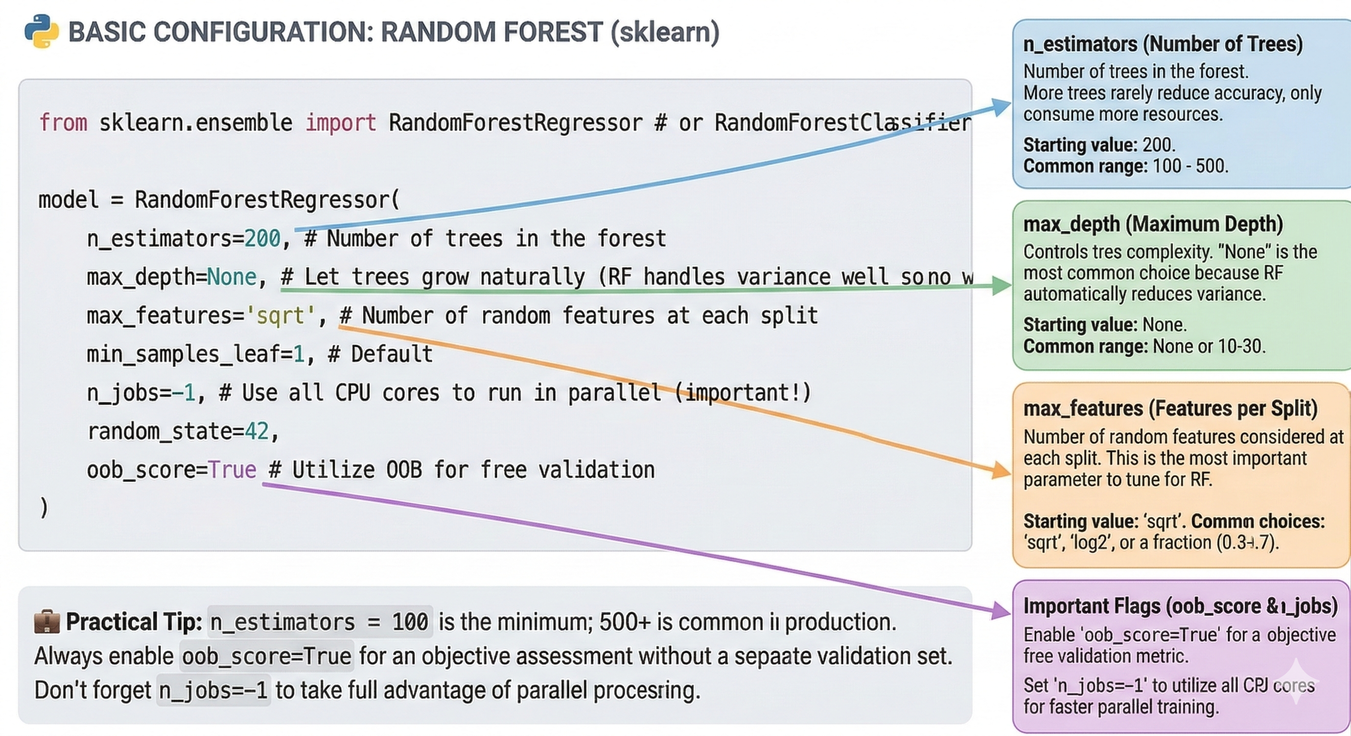
Figure 35. Random Forest needs less tuning thanks to good defaults.
7.3 Basic Configuration for XGBoost
This is the most complex part. XGBoost is like an F1 racing car: extremely fast, extremely powerful, but requires a highly skilled driver.
Declaration form (Python xgboost):
import xgboost as xgb

model = xgb.XGBRegressor(     # or XGBClassifier
    n_estimators=1000,        # Set high number, but will stop early thanks to Early Stopping
    learning_rate=0.05,       # Learning rate: Slow but steady
    max_depth=5,              # Shallow trees
    subsample=0.8,            # Only use 80% of data per tree (anti-overfit)
    colsample_bytree=0.8,     # Only use 80% of features per tree
    reg_lambda=1,             # L2 Regularization
    early_stopping_rounds=50, # If 50 rounds without improvement -> STOP IMMEDIATELY
    random_state=42,
    n_jobs=-1
)

# Training with Early Stopping (MANDATORY)
model.fit(
    X_train, y_train,
    eval_set=[(X_valid, y_valid)], # Need validation set to know when to stop
    verbose=False
)
Baseline values table:
| Hyperparameter | Baseline Value | Common Range | Notes |
|---|---|---|---|
| n_estimators | 1000 | 100 - 5000 | Always set high and let Early Stopping decide the stopping point. |
| learning_rate | 0.05 | 0.01 - 0.3 | Lower → more accurate → needs more trees. |
| max_depth | 5 | 3 - 10 | XGBoost prefers shallow trees (very different from RF). |
| subsample | 0.8 | 0.5 - 0.9 | Decrease to increase randomness (anti-overfit). |
Tips from practice:
- Always use Early Stopping! This is an unwritten rule. Never guess the number of trees
n_estimators. - There's an inverse relationship:
learning_rate × n_estimators ≈ constant. If you halve Learning Rate, be prepared for the number of trees (and training time) to double. - Quick strategy: Start with
learning_rate = 0.1to run quick experiments. After finalizing other parameters, reduce to0.01for the final model to squeeze out every bit of accuracy.
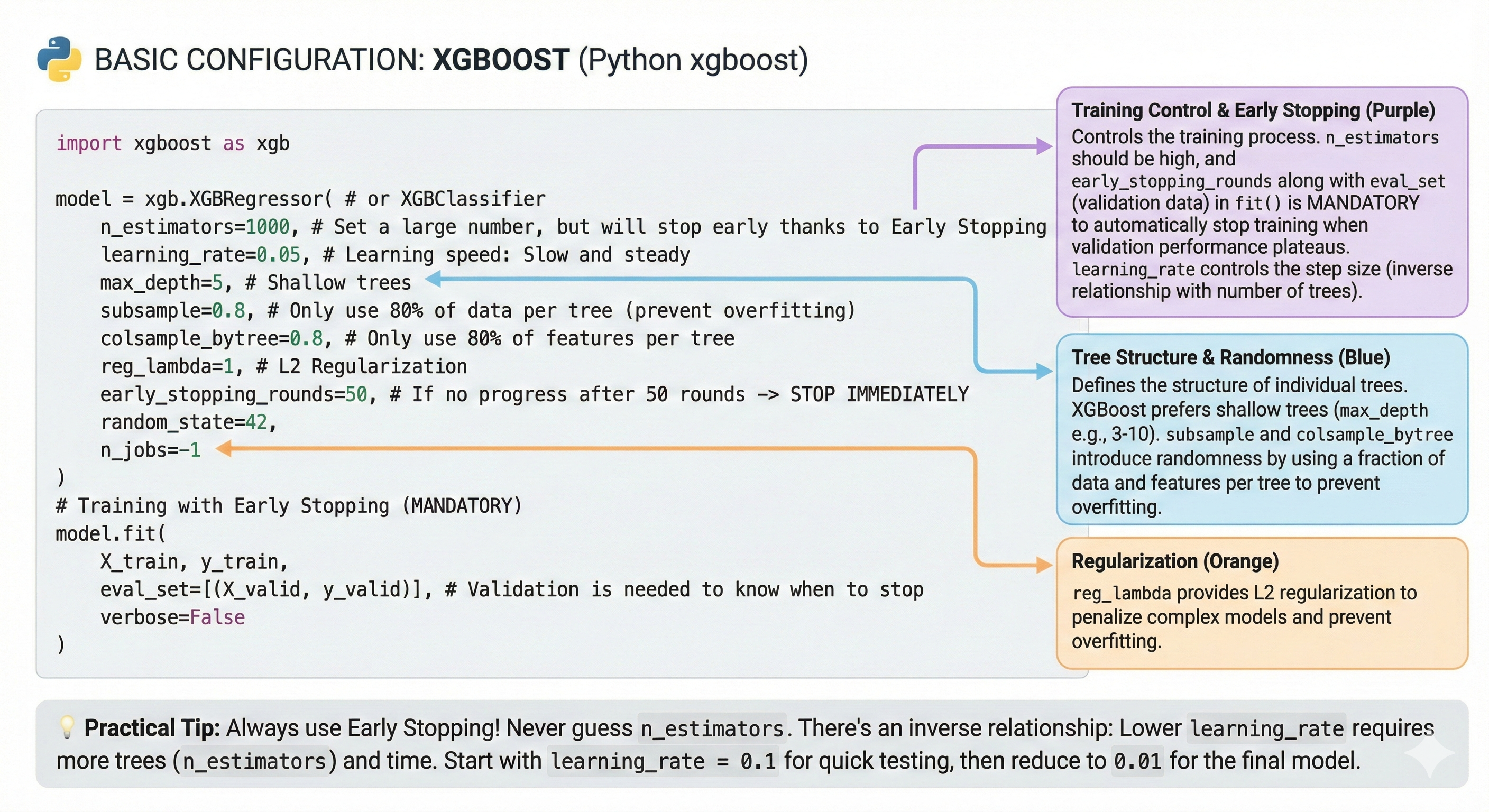
Figure 36. XGBoost has many parameters to tune, start from defaults.
7.4 Quick Comparison of 3 Model Configurations
To summarize, let's look at the comparison table below to see the differences in configuration philosophy:
| Parameter | Decision Tree | Random Forest | XGBoost |
|---|---|---|---|
| Number of sub-models | 1 | n_estimators (100-500) | n_estimators (100-5000) |
| Typical depth | 5-15 (Moderate) | None (Very deep - Full) | 3-7 (Very shallow) |
| Learning rate | N/A | N/A | 0.01 - 0.1 (Most important) |
| Stopping mechanism | N/A | Not needed | Early Stopping (Mandatory) |
| Overfitting risk | High | Low | High (if not tuned) |
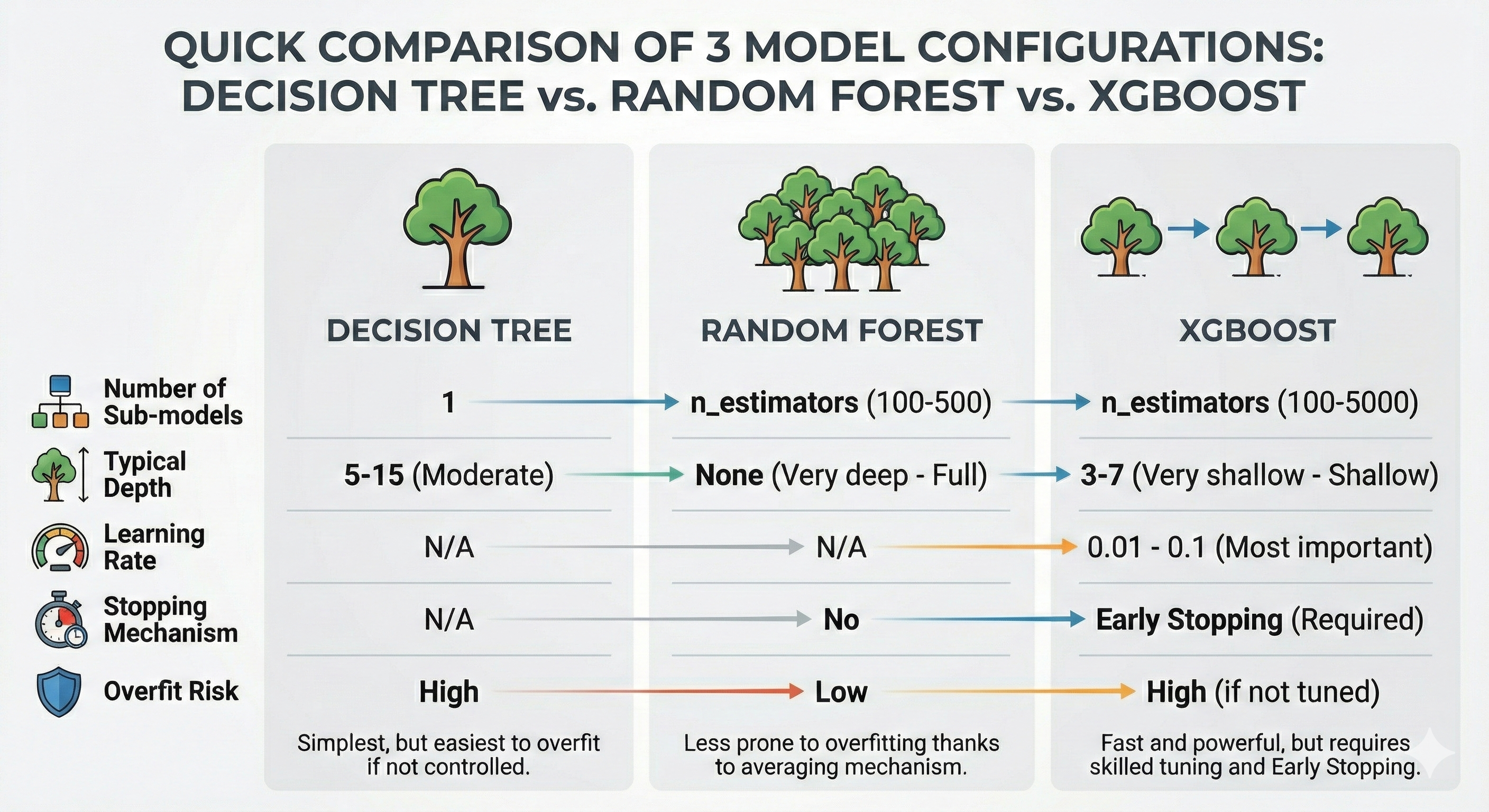
Figure 37. Trade-off comparison: Decision Tree is simple, XGBoost is powerful but needs more tuning.
7.5 Recommended Tuning Process
Don't try randomly (random guess). Tune according to this scientific process to save time:
-
Step 1: Baseline with Defaults. Run the model with default parameters to have a comparison benchmark.
-
Step 2: Tree Structure. Fix
learning_rate=0.1. Focus on finding optimalmax_depthandmin_child_weight. Always use Early Stopping. -
Step 3: Randomization & Regularization. Tune
subsample,colsample_bytreeandreg_lambdato reduce overfitting. -
Step 4: Fine-tune Learning Dynamics. After having a good framework, lower
learning_rateto very low (0.01 - 0.05) and increasen_estimatorsfor the model to converge to the optimal point. -
Step 5: Final Evaluation. Evaluate one last time on the Test set (this set must have been hidden from the beginning until now).
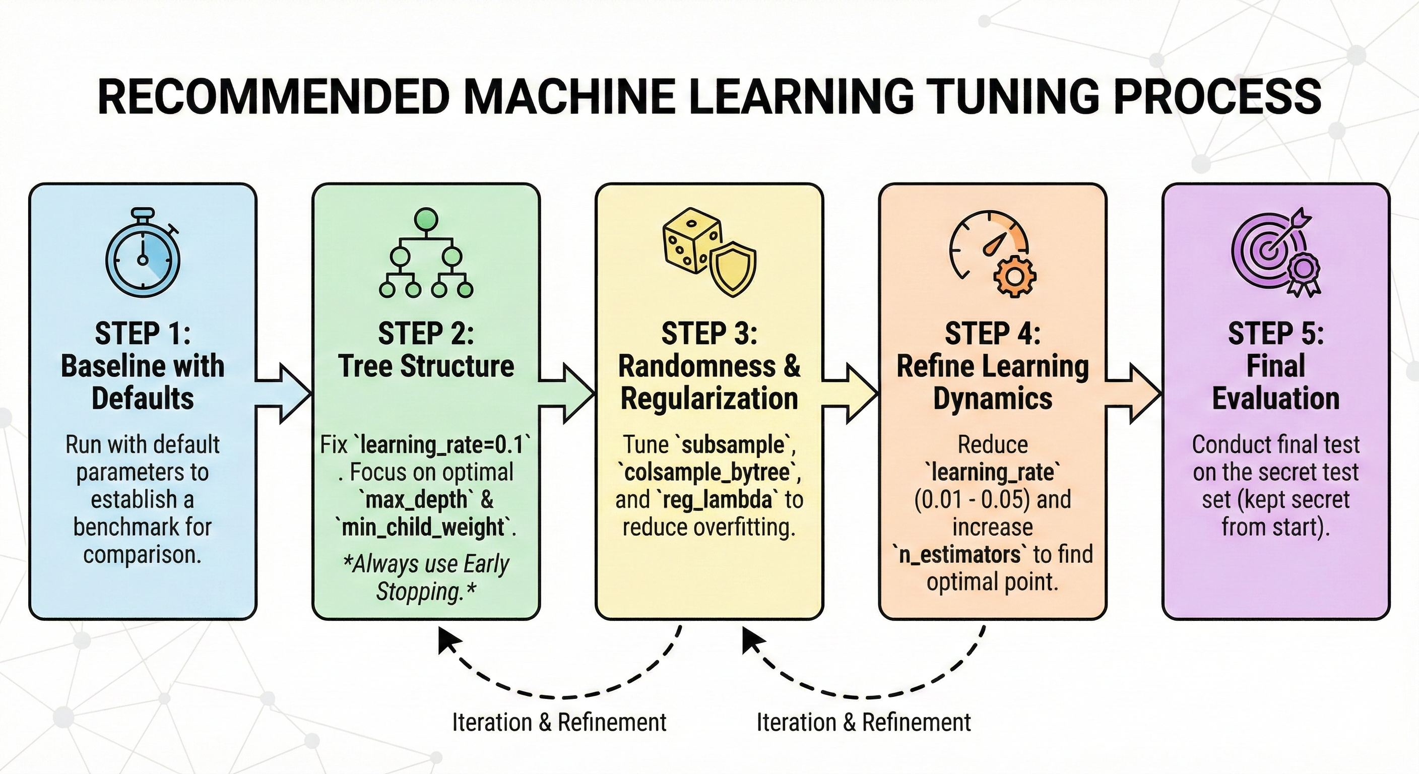
Figure 38. Tune from structure to regulation and learning dynamics.
VIII. Summary & Conclusion
We've traveled a long journey together, from the simplest concepts of "Wisdom of the Crowd" to complex techniques like Gradient Boosting or time series handling. To close this series of articles, I want to send you the most important takeaways — the baggage that will follow you throughout your Data Science career.
8.1 Five Golden Keys (Key Takeaways)
Amidst the vast ocean of knowledge, if you happen to forget all the mathematical formulas, just remember these 5 core principles well:
8.1.1. The Nature of Evolution
- Decision Tree: Is the foundational brick, easy to understand, easy to explain but "psychologically weak" (high Variance), very easily affected by noisy data.
- Random Forest (Bagging): Solves the problem with "quantity". Hundreds of trees voting together makes results stable and robust (Reduces Variance). This is the choice of Safety.
- XGBoost (Boosting): Solves the problem with "error correction". Later trees correct earlier trees' mistakes, helping the model achieve extremely high accuracy (Reduces Bias). This is the choice of Performance.
8.1.2. Model Selection Strategy
- Do you need a model that runs fast, requires little tuning, with good enough results to serve as a comparison baseline? → Call on Random Forest.
- Do you need to squeeze out every last 0.1% accuracy to compete or optimize products? → Use XGBoost.
8.1.3. Tuning Philosophy
- With Random Forest: Don't hesitate to increase the number of trees (
n_estimators). Focus on tuning the number of features per split (max_features). - With XGBoost: "Slow but steady" is the best strategy. Low learning rate (small
learning_rate) combined with a large number of trees (and Early Stopping) always brings the best results.
8.1.4. The Greatest Enemy: Overfitting
- Random Forest is hard to overfit thanks to the averaging mechanism, but it's not immortal.
- XGBoost easily overfits due to the overly thorough learning mechanism. Always prepare defense "armor" layers: shallow trees (low
max_depth), random sampling (subsample), and model penalization (reg_lambda).
8.1.5. The Time Trap
In Time Series, the future is not allowed to be revealed to the past. Forget random K-Fold and make friends with Walk-Forward Validation. Be careful with overlapping features between Train and Test sets.
8.2 Connection to Blog 1
Do you remember the story about Gradient (Derivative) in the first blog post? It's not just dry theory on paper.
Throughout this series, we've seen that Gradient is the "perpetual engine" operating inside XGBoost. Each new tree generated is guided by the Gradient of the loss function – it tells the model which direction to go to reduce error fastest. Understanding Gradient helps you understand why learning_rate is so important: it controls the stride length when we rush downhill to find the optimal point.
8.3 Conclusion: Tools and Mindset
Finally, I want to remind you that: Random Forest or XGBoost, no matter how powerful, are just tools. A sharp sword in the hands of someone who doesn't know martial arts also becomes useless, even causing injury to themselves.
The real value of a Data Scientist doesn't lie in typing the command import xgboost. That value lies in Mindset:
- Knowing how to look at raw data and tell its story.
- Knowing how to create smart features that the model can understand.
- Knowing how to choose the right metric for the problem.
- And most importantly, knowing when the model is "rote learning" and knowing when to stop.
I hope this series of articles has helped you build that thinking foundation. The road ahead is yours, take data as raw material and turn these algorithms into practical solutions. Wishing you success!
Chưa có bình luận nào. Hãy là người đầu tiên!