1. The Weekend Movie-Picking "Obsession" and the Birth of Recommender Systems
The weekend arrives. You open Netflix — or any streaming platform you're paying a monthly subscription for — stretch out on the sofa, and start scrolling. Scrolling past hundreds of colorful posters, skimming a few descriptions, clicking on a trailer then backing out, and scrolling again. Fifteen minutes go by. Thirty minutes. An hour. In the end, you close the app, open TikTok to watch some short clips to kill time, then go to sleep — without watching a single movie.
Sound familiar? You're not alone. This is a well-documented phenomenon in the product world: the paradox of choice — when there are too many options, people don't become happier; instead, they feel overwhelmed and end up choosing nothing at all.

The Paradox of Choice — the more movies available, the harder it is to choose.
Source: AI-generated illustration.
For entertainment platforms, this problem is a real headache. Content libraries keep expanding — tens of thousands of movies, overlapping genres, hard-to-distinguish titles. Meanwhile, every person has completely different tastes: some love Korean horror, others are into science documentaries, and some only watch comedies to unwind. The only thing they have in common is that nobody wants to spend hours just finding a movie to watch. When the search experience becomes exhausting, users leave — and that's the last thing any platform wants.
So how do we solve this? The answer lies in Recommender Systems.
Every time Netflix suggests "Because you watched Inception", or Spotify creates a "Discover Weekly" playlist, or an e-commerce platform recommends "Products you might like" — behind the scenes, a Recommender System is quietly at work. More specifically, the method we use in this project is Collaborative Filtering. The core idea is very intuitive: if you and a stranger have liked the same movies in the past, then movies that person enjoyed but you haven't seen yet are likely a good fit for you too. The system doesn't need to know who you are or what genres you prefer — it only needs behavioral data: who watched what, and how many stars they gave it. From there, it infers each user's level of interest in each movie and delivers truly personalized recommendations. Thanks to this, users no longer have to scroll through hundreds of titles — relevant suggestions appear almost instantly.
And that's exactly what our team decided to build from scratch.
Project Overview
In this project, we build an end-to-end pipeline: going from raw data all the way to an interactive demo that allows users to look up personalized movie recommendations. The input data is MovieLens 33M — a classic dataset in the Recommender System field, containing approximately 33 million ratings from hundreds of thousands of real users, spanning over 86,000 movies.
The entire process is deployed on Apache Spark and Delta Lake, enabling stable large-scale data processing that's ready to scale in a production environment. Architecturally, we apply the Medallion model (Bronze → Silver → Gold) to clearly separate each step: from ingesting raw data, to cleaning and exploration, to feature engineering for model training. The core algorithm is ALS (Alternating Least Squares) from Spark MLlib — a Collaborative Filtering method optimized for distributed data — combined with grid search and cross-validation to find the best hyperparameters. The result: a model achieving RMSE ≈ 0.78, an improvement of approximately 26% over the baseline of global mean prediction. Finally, a Streamlit demo is built to display the top 10 recommended movies for each user, integrated with TMDB posters to enhance the visual experience.

Pipeline overview: MovieLens → Medallion (Bronze/Silver/Gold) → ALS Model → Recommendation Demo.
Source: Authors.
As you can see, behind the seemingly simple suggestions on your screen lies an entire journey of large-scale data processing combined with the right machine learning algorithm. In the following sections, we'll walk through each stage of that journey: starting with how MovieLens data is organized and processed through the Medallion architecture; then the "brain" of the system — the ALS algorithm; followed by how the model is packaged into an interactive demo; and finally, lessons learned and future directions. Let's begin with the data story.
2. Data Pipeline: The Combination of Apache Spark, Delta Lake, and Medallion Architecture
In the world of data, raw data is like unrefined ore — it holds potential value but cannot be used directly. To transform 33 million movie rating records into clean data ready for machine learning algorithms, we need a well-structured processing pipeline. This section walks through each technology choice and how data flows through the system.
2.1. The MovieLens Dataset — The Classic "Training Ground" for Recommender Systems
Before building any model, we need data. And in the Recommender System field, there's one dataset considered the "gold standard" — that's MovieLens, published by the GroupLens research group at the University of Minnesota.
The version we use is MovieLens 33M, which includes approximately 33 million ratings from hundreds of thousands of real users, spanning over 86,000 movies. Each record contains core information: which user watched which movie, how many stars they gave it (on a 0.5–5.0 scale), and when the rating was submitted. There's also supplementary information such as movie genres, release years, and user-generated tags.
Why is MovieLens so popular? Because it's large enough to present real-world challenges — sparse matrices, skewed distributions, long-tail effects — yet also clean enough to let you focus on building models instead of spending weeks fixing data errors.

MovieLens 33M dataset structure — main tables and their relationships.
Source: Authors.
2.2. Why Apache Spark Instead of Pandas?
This is a question anyone working with data will ask: "MovieLens is only a few GB — Pandas can handle it just fine. Why bother with Spark?"
The answer comes down to two words: forward thinking.
True, with a dataset of a few million records, Pandas is perfectly capable. But Pandas operates on a single machine's RAM — when data grows to billions of rows (say, a streaming platform with 200 million users), memory simply won't be enough. Apache Spark solves this through distributed processing: splitting data into smaller partitions, processing them in parallel across multiple nodes, then aggregating the results.
More importantly, Spark MLlib — the built-in Machine Learning library — provides an ALS algorithm optimized for distributed data. This means from data pipeline to model training, everything stays within the same ecosystem, with no need to switch between tools.
We chose Spark not because the current data is too large, but because we wanted to build a pipeline that's ready to scale — when data grows 100x, there's no need to rewrite everything from scratch.
2.3. Why Delta Lake?
Saving data as plain CSV or Parquet sounds simple, but in practice, it comes with many risks: a write operation fails midway, data becomes inconsistent between runs, or you can't roll back to a previous version when you discover a mistake. Delta Lake acts as a protective layer on top, delivering three key benefits: ACID Transactions ensure data writes are always atomic — no "half-written" files; Time Travel allows you to roll back to previous data versions, which is invaluable for debugging; and Schema Enforcement prevents data with mismatched formats from entering the system.
In this project, every data layer (Bronze, Silver, Gold) is stored as a Delta Table — making the entire pipeline reproducible and auditable at any time.
2.4. Medallion Architecture: Three Layers of Data Refinement
Data in this project is organized according to the Medallion Architecture — a popular model in Data Engineering that divides the processing flow into three layers with increasing levels of refinement:
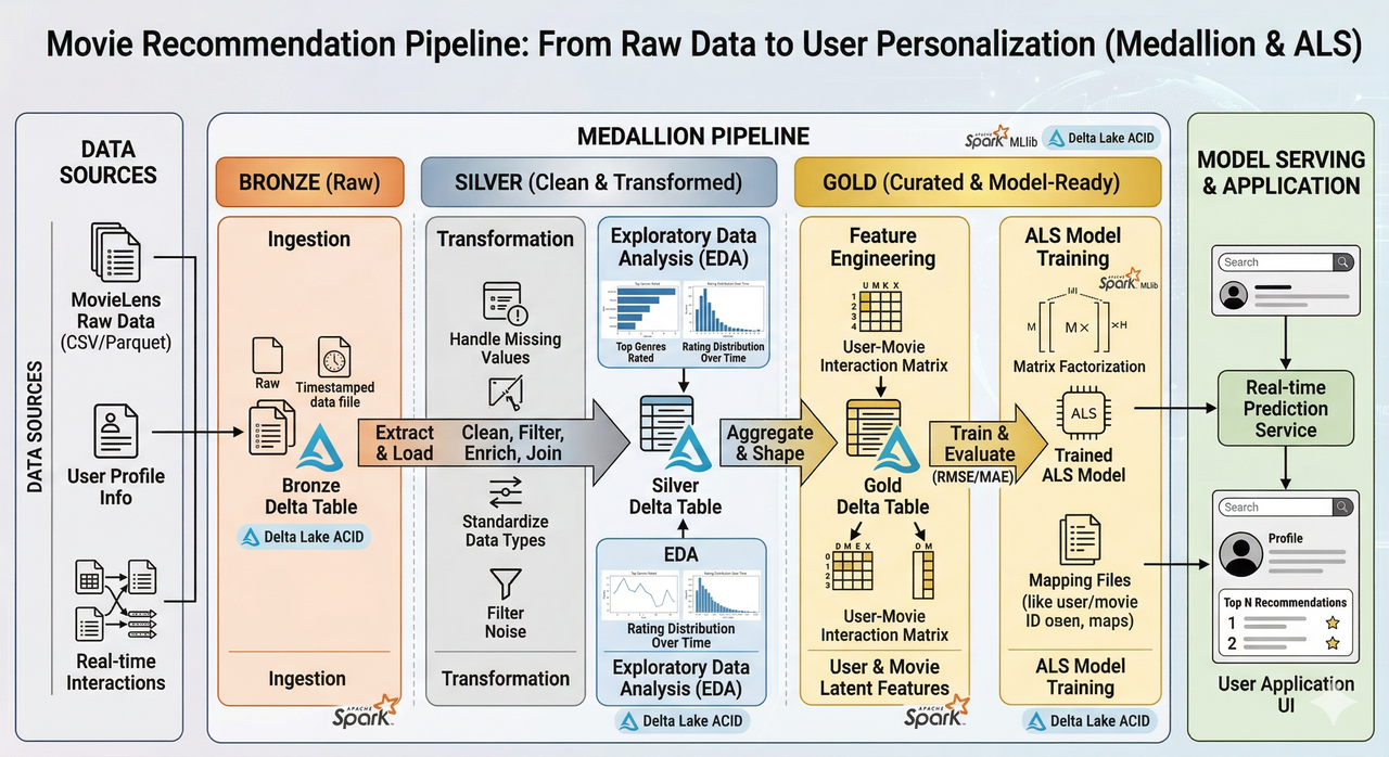
Data processing flow from Raw to ALS Model through the Medallion architecture.
Source: AI-generated illustration.
Bronze Layer — Raw Data
This is the "raw materials" layer. We ingest all original CSV files from MovieLens into Delta Tables, along with metadata (ingestion timestamp, source filename, batch ID) for traceability. The key point: data at this layer is kept as-is, with no modifications — the goal is to have a complete copy so the entire process can be reproduced if needed.
Instead of letting Spark infer data types automatically (inferSchema), we explicitly define the schema for each table:
# Explicit schema definition — no inferSchema
schemas = {
    "ratings": StructType([
        StructField("userId",    IntegerType(), True),
        StructField("movieId",   IntegerType(), True),
        StructField("rating",    DoubleType(),  True),
        StructField("timestamp", LongType(),    True),
    ]),
    # ... similarly for movies, tags, links, genome-scores, genome-tags
}

# Ingest with metadata tracking
def ingest_to_bronze(file_key, schema):
    df = spark.read.option("header", "true").schema(schema).csv(csv_file)
    df_with_meta = (
        df.withColumn("ingest_time", current_timestamp())
          .withColumn("source_file", lit(f"{file_key}.csv"))
          .withColumn("batch_id",    lit(batch_id))
    )
    df_with_meta.write.format("delta").mode("overwrite").save(output_path)
Silver Layer — Cleaning and Standardization
Before cleaning, we perform EDA (Exploratory Data Analysis) on the Bronze data to understand the data's "ailments." Some key findings from the EDA process:
- Left-skewed rating distribution — users tend to give high scores (average ~3.5/5). This will be addressed through user-bias normalization in the Gold layer.
- Long-tail distribution for both users and movies — most users rate very few movies, and most movies have very few ratings. This forms the basis for deciding filtering thresholds in the Gold layer.
- Extremely sparse User-Item matrix (~99.7% empty cells) — a classic characteristic of recommendation problems, and also the reason why ALS (matrix factorization) is more suitable than other methods.

Left-skewed rating distribution — 4.0 stars has the highest proportion (26.1%), confirming users' tendency toward positive ratings.
Source: Authors' analysis from MovieLens 33M data.

Long-tail distribution: most users rate very few movies. With a filtering threshold of ≥ 15 ratings (dashed line), 76.8% of users are retained.
Source: Authors' analysis from MovieLens 33M data.
Based on these findings, the Silver layer performs three main tasks: removing duplicate records (keeping the most recent rating), extracting information from movie titles (separating the clean title from the release year), and standardizing data types.
For example, with the ratings table, instead of using a simple dropDuplicates() (which keeps a random record), we use a Window function to ensure we always keep the most recent rating:
# Dedup ratings — keep the most recent rating per (userId, movieId)
window_latest = Window.partitionBy("userId", "movieId") \
                      .orderBy(col("timestamp").desc())

silver_ratings = (
    df_ratings_cast
    .withColumn("_rn", row_number().over(window_latest))
    .filter(col("_rn") == 1)
    .drop("_rn")
)
For the movies table, original movie titles are formatted as "Toy Story (1995)" — we split them into title_clean = "Toy Story" and release_year = 1995, while also converting the genre string "Action|Adventure" into an array ["Action", "Adventure"] for downstream analysis.
Gold Layer — Model-Ready Data
The Gold layer is where data undergoes its final refinement before being fed into the ALS algorithm. Here, we perform three main feature engineering steps, all justified by EDA results:
- Noise filtering: removing users with fewer than 15 ratings and movies with fewer than 10 ratings — these records carry signals too weak for collaborative filtering.
- Time decay weighting: recent ratings are assigned higher weights than older ones, reflecting the reality that user preferences change over time.
- User-bias normalization: normalizing ratings by each user's average — because some users always give 5 stars while others are strict and only give 2–3 stars; without this adjustment, the model would be biased.
After the Gold layer, the data is clean, enriched with additional features, and ready to become the "fuel" for the ALS algorithm in the next section.
3. Decoding the System's "Brain" — The Collaborative Filtering Algorithm (ALS)
The data has passed through the three refinement layers of the Medallion architecture. After noise filtering and feature engineering in the Gold layer, we're left with a high-quality dataset — ready to "teach" a computer to understand people's movie-watching preferences. But how exactly does a computer "learn" from tens of millions of rating numbers? This is where the system's "brain" comes into play.
3.1. Collaborative Filtering and Its Mathematical Essence (Matrix Factorization)
The core idea of Collaborative Filtering was introduced in Section 1: if you and a stranger have liked the same movies in the past, the system will recommend movies that person enjoyed but you haven't seen yet. But to turn this intuitive idea into an algorithm, we need to dive a bit deeper into the mathematics.
The first step is to construct the User-Item matrix — a massive table where rows represent users ($u$), columns represent movies ($i$), and each cell contains the rating ($r_{ui}$) that user gave to that movie. The problem is that this matrix is extremely sparse — EDA from the previous section showed ~99.7% empty cells, since each person only watches and rates a very small fraction of the tens of thousands of available movies.
How do we "fill in" those empty cells? This is where Matrix Factorization comes into play. The idea is to "compress" the large matrix $R$ into the product of two smaller matrices:
- $U$ (User Feature Matrix): Dimensions $M \times k$
- $V$ (Movie Feature Matrix): Dimensions $N \times k$
Where $k$ is the number of latent dimensions — think of it as the number of "psychological aspects" the system uses to describe preferences. For example, one dimension might represent how much someone likes action movies, another might capture a preference for complex storylines, etc. The predicted rating for user $u$ on movie $i$ is the dot product:
$$\hat{r}_{ui} = u_u^T v_i$$
To find the best matrices $U$ and $V$, we need to minimize the Loss Function — measuring the deviation between predictions and actual values, combined with L2 Regularization (parameter $\lambda$) to prevent overfitting:
$$L(U, V) = \sum_{(u,i)} (r_{ui} - u_u^T v_i)^2 + \lambda \left( \sum_u ||u_u||^2 + \sum_i ||v_i||^2 \right)$$
Where:
- $r_{ui}$: The actual rating that user $u$ gave to movie $i$.
- $u_u$: The latent feature vector representing the preferences of user $u$.
- $v_i$: The latent feature vector representing the attributes of movie $i$.
- $\lambda$ (Lambda): Regularization parameter — the larger it is, the simpler the model, reducing the risk of overfitting.
- $||u_u||^2$ and $||v_i||^2$: The squared L2 Norms of the vectors.
3.2. Why ALS? And How It's Implemented on Spark MLlib
The optimization problem for the Loss function above isn't straightforward — since both $U$ and $V$ are unknowns, the Loss function is not convex. This is where the ALS (Alternating Least Squares) algorithm shows its elegance: instead of trying to solve for both matrices simultaneously, ALS fixes one matrix and optimizes the other, then alternates. Specifically:
- Fix $U$: the Loss function becomes a quadratic equation in $V$ → solvable via Least Squares.
- Fix $V$: the Loss function becomes a quadratic equation in $U$ → solved similarly.
- Repeat until convergence.
The crucial point: when one side is fixed, the computations for each user (or each movie) are independent of each other — and this is exactly why ALS is a perfect match for Spark. Spark can split the work, distribute it across multiple nodes for parallel computation, then aggregate the results. This is also why Spark MLlib chose ALS as its default recommendation algorithm.
Implementation on Spark MLlib is quite concise:
from pyspark.ml.recommendation import ALS

als = ALS(
    userCol="userId",
    itemCol="movieId",
    ratingCol="rating",
    coldStartStrategy="drop",   # skip users/movies not in the training set
    nonnegative=True,           # keep latent factors non-negative → easier to interpret
)
However, the model's effectiveness depends heavily on choosing the right hyperparameters. We set up a Grid Search combined with 3-fold Cross Validation to find the best parameter combination:
from pyspark.ml.tuning import CrossValidator, ParamGridBuilder

param_grid = (
    ParamGridBuilder()
    .addGrid(als.rank,     [15, 20])     # number of latent features k
    .addGrid(als.regParam, [0.05, 0.1])  # regularization parameter λ
    .addGrid(als.maxIter,  [10, 15])     # number of iterations
    .build()
)

cv = CrossValidator(
    estimator=als,
    estimatorParamMaps=param_grid,
    evaluator=rmse_evaluator,
    numFolds=3,
    parallelism=2,   # run 2 models in parallel — safe for 14GB RAM
)
A total of 24 model fits (8 parameter combinations × 3 folds). The best parameters returned by Cross Validation:
rank = 20— movie-watching preferences are quite complex, requiring 20 "latent dimensions" to describe.regParam = 0.05— moderate regularization.maxIter = 15— enough iterations to converge.
3.3. Evaluating Training Results
To evaluate the model, we use three metrics common in regression problems:
-
MSE (Mean Squared Error):
$$MSE = \frac{1}{N} \sum_{i=1}^{N} (y_i - \hat{y}_i)^2$$ -
RMSE (Root Mean Squared Error):
$$RMSE = \sqrt{\frac{1}{N} \sum_{i=1}^{N} (y_i - \hat{y}_i)^2}$$ -
MAE (Mean Absolute Error):
$$MAE = \frac{1}{N} \sum_{i=1}^{N} |y_i - \hat{y}_i|$$
Where:
- $y_i$: The actual rating.
- $\hat{y}_i$: The predicted rating.
Results on the test set:
| Metric | ALS Model | Baseline (Global Mean) | Improvement |
|---|---|---|---|
| RMSE | 0.7834 | 1.0607 | 26.1% |
| MSE | 0.6137 | — | — |
| MAE | 0.6002 | 0.8399 | — |
What does MAE = 0.6002 mean in practice? On average, each prediction deviates by about 0.6 stars from the user's actual rating. If the system predicts you'll rate a movie 4.5 stars, the actual score is very likely to fall between 3.9 and 5.0 stars — a fairly acceptable margin of error.
To put this in context: the Global Mean Baseline — the simplest model, which takes the overall training set average and assigns it to every user-movie pair — yields an RMSE of 1.0607. The ALS algorithm reduces this to 0.7834, equivalent to a 26.1% improvement. This difference comes from the ability to factorize the matrix and discover unique latent features for each user, rather than treating everyone the same.

Prediction analysis: errors centered around 0 (left), model closely follows the perfect prediction line (center), MAE lowest in the mid-rating range (right).
Source: Authors' analysis from ALS model training results.
Looking at the analysis charts, we draw several observations: the error distribution is symmetric around 0, indicating the model is not systematically biased. However, the model tends to pull predictions toward the mean — predicting higher than actual for low-rated movies and lower than actual for high-rated movies. This is a common characteristic of matrix factorization when working with sparse and imbalanced data. Overall, the model performs stably in the mid-rating range (3.0–4.0) and could be further improved for extreme cases using advanced techniques — which we'll discuss in Section 5.
4. From Notebook to Demo — Packaging the Model into an Interactive Prototype
4.1. A Good Model in a Notebook Is Still Just a Notebook
The ALS model has been trained, achieving RMSE = 0.7834, a 26% improvement over the baseline. But a model sitting in a Jupyter Notebook is no different from a great recipe that nobody gets to taste. To validate the results more visually — and to get hands-on experience with the "serving" step in the ML lifecycle — we decided to package it into an interactive demo using Streamlit.
To be clear: this is a proof-of-concept prototype, not a production application. Recommendations are precomputed for a fixed set of users and saved as a static JSON file — there's no ability to handle new users, no real-time updates, and users must enter a User ID rather than logging in with a real account. But for the purpose of this project — experiencing the full pipeline from raw data to an interface you can interact with — it has served its role well.
4.2. The Export and Serving Process
Our strategy is precompute — calculating all recommendations in advance for 30,000 users, saving them as a JSON file, so the demo only needs to look up results without running Spark at serving time. This process consists of four steps:
Step 1 — Reload the model and data. The ALS model saved from training is loaded back, along with the Silver/Gold tables:
# Load the trained ALS model
best_model = ALSModel.load(model_path)

# Load data from Silver & Gold
df_ml      = spark.read.format("delta").load(f"{gold_path}/gold_train_features_ml")
df_movies  = spark.read.format("delta").load(f"{silver_path}/movies_clean")
df_ratings = spark.read.format("delta").load(f"{silver_path}/ratings_clean")
df_links   = spark.read.format("delta").load(f"{silver_path}/links_clean")
Step 2 — Generate top 10 recommendations for all users. We select the first 30,000 users (sorted by userId for reproducibility), then use recommendForUserSubset to generate recommendations:
# Select 30,000 users for serving
target_users = (
    df_ml.select("userId").distinct()
    .orderBy(asc("userId"))
    .limit(30000)
)

# Generate top-10 recommendations for each user
user_recs = best_model.recommendForUserSubset(target_users, 10)
Step 3 — Post-processing and joining metadata. Predicted scores are clipped to the [0.5, 5.0] range to avoid unreasonable values, then movie information (title, genre, community score) is joined to each recommendation:
final_serving = (
    user_recs
    .withColumn("rec", explode("recommendations"))
    .select(
        col("userId").cast("string"),
        col("rec.movieId").alias("movieId"),
        # Clip predicted scores to valid range [0.5, 5.0]
        F.least(F.lit(5.0), F.greatest(F.lit(0.5),
            F.round(col("rec.rating"), 2)
        )).alias("pred_rating")
    )
    .join(
        df_movie_metadata.select(
            "movieId", "title_clean", "genres", "tmdbId", "avg_rating", "release_year"
        ),
        "movieId", "left"
    )
)
Step 4 — Write to JSON for serving. Results are grouped by User ID and saved as serving_recs.json. From this point, whenever a user enters their ID in the demo, Streamlit simply looks up the right key — instant response, no Spark required:
# Group recommendations by userId → list of recommendations
serving_df = (
    final_serving
    .groupBy("userId")
    .agg(
        collect_list(
            struct("movieId", "title_clean", "genres",
                   "pred_rating", "avg_rating", "tmdbId", "release_year")
        ).alias("recs")
    )
)

# Export to JSON
with open(f"{assets_path}/serving_recs.json", "w", encoding="utf-8") as f:
    json.dump(serving_dict, f, ensure_ascii=False)
When the Streamlit demo starts, JSON files are loaded into memory and cached with @st.cache_data, ensuring all subsequent lookups take only a few milliseconds:
@st.cache_data
def load_assets():
    with open(os.path.join(assets_path, "model_info.json"), "r") as f:
        model_info = json.load(f)
    with open(os.path.join(assets_path, "serving_recs.json"), "r") as f:
        serving_data = json.load(f)
    return model_info, serving_data
4.3. The CineMatch Demo
The entire process above is packaged into the CineMatch demo, built on the Streamlit platform. The goal is not a polished product, but a prototype sufficient to visualize the ALS model's results in an interactive format. The interface is designed with a modern dark mode aesthetic with a cinematic feel. The demo has two main features, clearly separated into two tabs:
"Personal Recommendations" Tab — this is the core feature. Users enter their User ID, the system looks it up in serving_recs.json and returns a list of suitable movies, with optional genre filtering:
if submitted:
    uid = str(user_id_input).strip()
    if uid not in all_recs:
        st.markdown(f"User ID {uid} is not in the precomputed set...")
    else:
        recs = all_recs[uid]

        # Filter by genre if user selected any
        if selected_genres:
            recs = [
                r for r in recs
                if any(g in (r.get("genres") or "") for g in selected_genres)
            ]

        # Display in a 5-column grid
        cols_per_row = 5
        for row_start in range(0, len(recs), cols_per_row):
            row_movies = recs[row_start : row_start + cols_per_row]
            cols = st.columns(cols_per_row)
            for col, movie in zip(cols, row_movies):
                with col:
                    render_movie_card(movie, show_pred=True)
Each movie card displays the poster, title, release year, genre, the predicted score specific to that user, and the community average score. For example, for User 510, the system recommends movies like Forrest Gump (4.38 score), Aladdin (4.25 score), and Koko-di Koko-da (4.66 score) — reflecting that user's personal preferences:

Recommendations for User 510 — each movie card displays the poster, predicted score, and community score.
Source: CineMatch Demo.
"Search Movies" Tab — allows searching for movies by name and filtering by genre. The results list is sorted using a formula that combines the average rating with the number of ratings, preventing movies with few ratings but abnormally high scores from appearing at the top. When no search keyword is provided, this tab defaults to displaying the top 10 highest-rated movies across the entire dataset:

"Search Movies" tab — top 10 highest-rated movies, sorted by Bayesian Average.
Source: CineMatch Demo.
A small but important detail for the user experience: each movie card needs a poster to display. The demo calls the TMDB API using the tmdbId stored in the metadata, with results cached for 1 hour to avoid redundant calls. If no API key is available or the call fails, the demo automatically uses a placeholder image to ensure the interface never breaks under any circumstances.
From a model sitting idle in a notebook, we've packaged it into an interactive demo — not a production application, but enough for anyone to open up, enter a User ID, and visually verify the recommendation results. But the journey doesn't stop here — in the final section, we'll reflect on the lessons learned and the next steps to make this system truly production-ready.
5. Lessons Learned and Future Directions
5.1. Looking Back: From CSV Files to a Working Recommendation Pipeline
Looking back at the entire project from start to finish, we've gone through a fairly complete journey of a real-world Data/ML project — not just stopping at "training a model and printing results in a notebook," but building an entire end-to-end pipeline from raw data to an interface that users can interact with.
Specifically, four core technical pillars were applied throughout the project:
First, large-scale data processing with Apache Spark. Instead of using Pandas — which only works well when data fits in a single machine's memory — we leveraged Spark for distributed data processing. With the current MovieLens dataset, Pandas would still "work," but the Spark architecture allows the system to be ready to scale when ratings grow to hundreds of millions or billions of rows without needing to rewrite code from scratch. This is designing for the future, not just for the present.
Second, building a professional Data Pipeline with Medallion Architecture and Delta Lake. Organizing data into three layers — Bronze → Silver → Gold — not only makes the pipeline easier to debug and maintain but also ensures data consistency and traceability (data lineage). Delta Lake adds critical features like ACID transactions and time travel, giving us confidence that data won't be corrupted or lost during processing. This is how Data Engineering teams at major companies operate their systems daily.
Third, applying Machine Learning algorithms — specifically Collaborative Filtering with ALS. We transformed a simple idea ("people with similar tastes will like similar movies") into a concrete mathematical model through Matrix Factorization. Spark MLlib provides an ALS implementation optimized for distributed processing, enabling efficient training even on large datasets. Evaluating the model using RMSE and MAE also gives us a quantitative view of prediction quality, rather than relying on intuition.
Fourth, taking the model out of the notebook and packaging it into an interactive demo. This is the step where many ML projects stall and never complete. Exporting the model, creating mapping files, and building a UI interface so users can actually interact with the recommendation system — this is the gap between a "notebook exercise" and a "prototype with an interface." Going from prototype to a real product requires many more steps — and that's exactly what Section 5.3 covers. Even at a small scale, this step gave us real-world experience with the model serving process.
5.2. Remaining Challenges
No system is perfect, and our recommendation system is no exception. There are several difficult problems that the current project hasn't fully addressed.
Cold Start Problem — "Enemy Number One" of Collaborative Filtering. This is the biggest challenge and an inherent limitation of the Collaborative Filtering approach. The system operates based on users' interaction history (ratings), so what happens when a brand-new user signs up and hasn't rated any movies? Or when a new movie is released with no ratings yet? In both cases, the User-Item matrix has no data for the model to "learn" from and provide meaningful recommendations. Currently, the system falls into a "don't know what to recommend" state for these cases — a significant gap if deployed at real-world scale, where new users are constantly joining.
Popularity Bias. Collaborative Filtering tends to recommend movies that have already been watched and highly rated by many people, inadvertently overlooking lesser-known films (niche films) that might actually be a perfect match for a user's taste. This leads to a "rich get richer" phenomenon — popular movies get recommended more and more, while lesser-known films gradually "sink" in the system.
Sparsity Problem. In practice, the number of movies each user has watched and rated represents only a tiny fraction of the total movies in the system. The User-Item matrix is therefore extremely sparse, with the vast majority of cells empty. When data is sparse, finding accurate latent features becomes more difficult, directly affecting recommendation quality.
Explainability. When the model recommends Movie A to User B, it's hard to clearly explain "why." The latent features in Matrix Factorization are abstract numerical vectors that don't carry specific semantic meaning like "action genre" or "director Christopher Nolan." This makes building user trust in the system challenging — users typically want to know the reason behind a recommendation, not just receive one.
5.3. Future Development Directions
Based on the challenges above, there are several clear directions for upgrading the system.
Combining Content-Based Filtering to create a Hybrid Model. This is the most natural next step. Instead of relying solely on users' rating behavior (Collaborative Filtering), we can supplement with movie content information — genres, directors, actors, synopses, and even posters and trailers. A Hybrid model combining both signal sources would partially address the Cold Start problem: even if a new user has no rating history, the system can still recommend based on genre preferences they select during registration, or based on content features of similar movies.
Experimenting with Deep Learning architectures. Modern Recommender Systems have gone far beyond traditional Matrix Factorization. Architectures like Neural Collaborative Filtering (NCF), Variational Autoencoders (VAE) for Recommendation, or even Transformer-based models (like SASRec — Self-Attentive Sequential Recommendation) can capture more complex non-linear relationships between users and movies. In particular, Sequential Recommendation models can leverage the temporal order of ratings to understand how user preferences change over time — something traditional ALS cannot do.
Deploying to the Cloud for true system scaling. Currently, the entire system runs in a local environment. To put the system into real-world operation with thousands or millions of users, we need to deploy on Cloud platforms like AWS, GCP, or Azure. More specifically, the data processing pipeline could run on services like AWS EMR or Databricks, model serving could be deployed via API endpoints with AWS SageMaker or GCP Vertex AI, and the entire retraining workflow could be automated using orchestration tools like Apache Airflow or Prefect.
Adding Implicit Feedback. In the current project, we use explicit feedback (ratings that users actively provide). However, in practice, the majority of user signals are implicit — views, watch time, pause behavior, adding to watchlists, or even abandoning a movie midway. Integrating these signals would help the model understand users' true preferences more deeply, rather than relying only on the occasions when they "cared enough" to leave a rating.
Looking at the big picture, this project is not merely an exercise in recommendation algorithms. It's a journey through the entire lifecycle of a data project: from collecting and processing raw data, exploring and cleaning data, training and evaluating models, to packaging everything into a prototype that users can interact with directly. Each step carries its own lessons, and more importantly, each unresolved challenge is the motivation to continue improving and developing the system in the future.
Connect With Us
If you're interested in this project, want to see the detailed code, or have any feedback — we'd love to hear from you!
Leave a comment below if you have questions, or if you've tried building your own recommendation system — we'd love to hear your story!
References
-
F. Maxwell Harper & Joseph A. Konecny, The MovieLens Datasets: History and Context, ACM Transactions on Interactive Intelligent Systems, 2015. — https://grouplens.org/datasets/movielens/
-
Yehuda Koren, Robert Bell & Chris Volinsky, Matrix Factorization Techniques for Recommender Systems, IEEE Computer, 2009.
-
Apache Spark Documentation — MLlib Collaborative Filtering (ALS). — https://spark.apache.org/docs/latest/ml-collaborative-filtering.html
-
Delta Lake Documentation — ACID Transactions, Time Travel, Schema Enforcement. — https://docs.delta.io/latest/index.html
-
Databricks, Medallion Architecture: Bronze, Silver, Gold. — https://www.databricks.com/glossary/medallion-architecture
-
Hu, Y., Koren, Y. & Volinsky, C., Collaborative Filtering for Implicit Feedback Datasets, IEEE ICDM, 2008.
-
Streamlit Documentation — Build and share data apps. — https://docs.streamlit.io/
-
TMDB (The Movie Database) API Documentation. — https://developer.themoviedb.org/docs
Chưa có bình luận nào. Hãy là người đầu tiên!