1. Introduction
"Out of every 1,000 songs released on Spotify, only about 6 can become a true HIT."
This means 99.4% of songs released - no matter how much effort, talent, or studio time is invested - never truly break through. So what makes that tiny fraction of songs reach the top? Is there a "magical" formula behind hit songs, or is success in music simply a JACKPOT in statistical probability?!
To explore this question, we will analyze the dataset "550k Spotify Songs - Audio, Lyrics and Genres" on Kaggle, which includes over 550 thousand songs along with characteristics such as artist information, music genres, and lyrics....
The goal of this article is to examine whether successful songs share common patterns and characteristics. For instance, does higher danceability, more energy, or a distinctive loudness level create a difference compared to the vast majority of other songs.
2. Dataset Explanation
In this article, we use a publicly available dataset on Kaggle:
Dataset "550k Spotify Songs - Audio, Lyrics and Genres": https://www.kaggle.com/datasets/serkantysz/550k-spotify-songs-audio-lyrics-and-genres/data
This dataset consists of two main files:
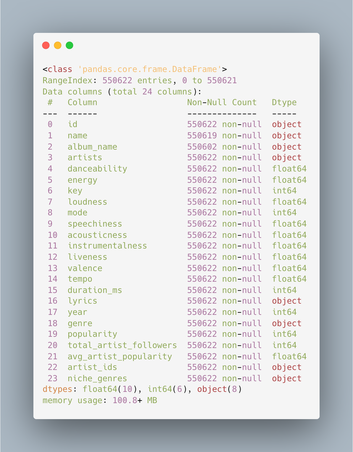
- songs.csv - containing 550,622 songs with 24 data columns, including features such as album name (album_name), artist name (artists), lyrics (lyrics),... and popularity score (popularity) on Spotify.
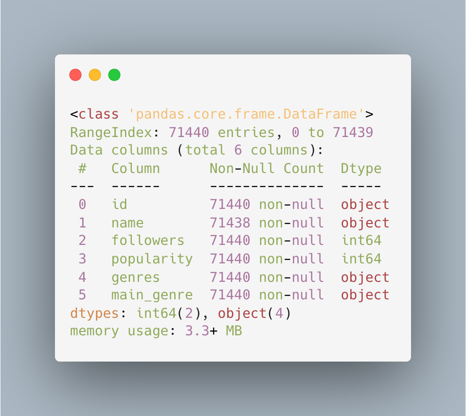
- artists.csv - containing 71,440 artists with 6 data columns, including follower count (followers), artist popularity (popularity), and main music genre (main_genre)...
songs.csv
artists.csv
3. Data Cleaning
3.1. Finding Data Problems
This is the most important step before analysis - detecting issues that could distort results.
3.1.1. Check for Missing Data
artists.csv
print("=== MISSING VALUES: artists.csv ===")
print(artists_raw.isnull().sum())
print(f"\nTotal rows: {len(artists_raw)}")
Missing values are minimal: only 2 missing values in the name column (0.003%). Since the ratio is under 5%, we can safely drop these rows directly.
songs.csv
print("=== MISSING VALUES: songs.csv ===")
print(songs_raw.isnull().sum())
print(f"\nTotal rows: {len(songs_raw)}")
Similarly, songs.csv has only 3 missing song names and 20 missing album names - negligible across 550,000+ records. Rows missing critical columns (name, artists, year, genre, popularity, danceability, energy, loudness, valence, tempo) will be dropped.
3.1.2. Check for Duplicates
artists.csv
print("=== DUPLICATES: artists.csv ===")
print(f"Duplicate IDs: {artists_raw.duplicated(subset=['id']).sum()}")
print(f"Duplicate names (exact): {artists_raw.duplicated(subset=['name']).sum()}")
name_lower = artists_raw['name'].str.strip().str.lower()
print(f"Duplicate names (case-insensitive): {name_lower.duplicated().sum()}")
- Duplicate IDs: 0
- Duplicate names (exact): 1,796
- Duplicate names (case-insensitive): 2,098
The case-insensitive name duplicates are quite significant - the same artist may appear under different casing (e.g., "the weeknd" and "The Weeknd"). These need to be resolved by keeping the record with the highest popularity score.
songs.csv
print("=== DUPLICATES: songs.csv ===")
print(f"Duplicate IDs: {songs_raw.duplicated(subset=['id']).sum()}")
songs_raw['_name_lower'] = songs_raw['name'].str.strip().str.lower()
songs_raw['_artists_lower'] = songs_raw['artists'].astype(str).str.strip().str.lower()
n_case_dups = songs_raw.duplicated(subset=['_name_lower', '_artists_lower']).sum()
print(f"Duplicate (song + artist, case-insensitive): {n_case_dups}")
songs_raw.drop(columns=['_name_lower', '_artists_lower'], inplace=True)
- Duplicate IDs: 0
- Duplicate song title + artist (case-insensitive): 50,056
Over 50,000 songs share the same title and artist - most likely from rereleases, compilation albums, or regional versions. Only the version with the highest popularity score is kept to avoid duplication.
3.1.3. Check for Outliers & Data Logic
# --- songs.csv ---
print("=== DATA LOGIC: songs.csv ===")
print(f"Popularity range: {songs_raw['popularity'].min()} - {songs_raw['popularity'].max()}")
print(f"Songs with popularity = 0: {(songs_raw['popularity'] == 0).sum()}")
print(f"Year range: {songs_raw['year'].min()} - {songs_raw['year'].max()}")
print(f"Duration range: {songs_raw['duration_ms'].min()/60000:.1f} - {songs_raw['duration_ms'].max()/60000:.1f} minutes")
# --- artists.csv ---
print("=== DATA LOGIC: artists.csv ===")
print(f"Popularity range: {artists_raw['popularity'].min()} - {artists_raw['popularity'].max()}")
print(f"Followers range: {artists_raw['followers'].min()} - {artists_raw['followers'].max()}")
- Popularity must be within the range 0–100. Values outside this range will be removed.
- Songs with popularity \= 0 are most likely unstreamed or inactive tracks. Before dropping: 402,974 rows, mean popularity 17.74. After dropping: 303,142 rows, mean popularity 23.58.
- Year range: The raw data spans from 1900–2025. Since the analysis focuses on modern music trends, we only keep songs from year 2000 onward.
3.1.4. Check Data Format
# --- artists.csv ---
print("=== DATA TYPES: artists.csv ===")
print(artists_raw.dtypes)
# --- songs.csv ---
print("=== DATA TYPES: songs.csv ===")
print(songs_raw.dtypes)
- Numeric columns (danceability, energy, key, loudness, mode, speechiness, acousticness, instrumentalness, liveness, valence, tempo, duration_ms, year, popularity, total_artist_followers, avg_artist_popularity) were converted to proper numeric types using pd.to_numeric(errors='coerce').
- The followers and popularity columns in artists.csv were also converted similarly, with invalid values replaced by 0.
3.2. Cleaning Steps
After identifying the problems, we applied the following cleaning steps:
artists.csv:
- Dropped 2 rows with missing artist names
- Checked for duplicate IDs (0 found)
- Resolved 2,097 case-insensitive duplicate names - kept the record with the highest popularity
- Converted followers and popularity to numeric types
- Filtered popularity to valid range [0, 100] (0 rows removed)
Result: 71,440 → 69,341 rows
songs.csv:
- Filtered year ≥ 2000 (550,622 → 453,033 rows)
- Dropped 3 rows missing data in critical columns
- Checked for duplicate IDs (0 found)
- Resolved 50,056 duplicate song title + artist records - kept the version with the highest popularity
- Converted columns to proper numeric types
- Created Status column (Flop / Average / Hit)
- Dropped songs with popularity \= 0 (402,974 → 303,142 rows)
- Converted duration_ms to minutes
Result: 550,622 → 303,142 songs, including 1,776 hits
Popularity Metric and Hit Classification
Each song in the dataset has a popularity score assigned by Spotify, ranging from 0 to 100. This metric is algorithmically calculated based on multiple factors such as total stream count, recency of streams, and other forms of user engagement.
To make this continuous metric easier to interpret for later analysis, we converted it into three categorical groups:
| Status | Popularity Range | Percentage (%) of Total |
|---|---|---|
| Flop | 0 – 30 | 69.13 |
| Average | 31 – 70 | 30.28 |
| Hit | 71 – 100 | 0.59 |
4. Feature Distribution
4.1. Distribution of Numerical Features by Status
To understand the differences between the Flop, Average, and Hit groups, we plotted distribution charts (histogram + KDE) for each audio feature, split by the 3 Status groups.
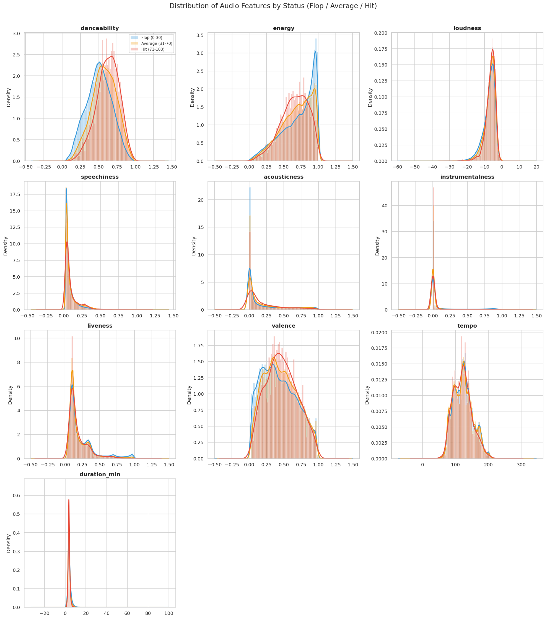
Observations:
- Danceability shows the most distinct difference between the three groups. The KDE curve for Hit songs shifts noticeably to the right, clustering around 0.55–0.75, while Flop songs spread wider with a lower peak. Songs with strong, steady rhythms are clearly more likely to achieve mainstream success.
- Instrumentalness has the strongest separation: all three groups concentrate near 0, but Flop songs have a long tail extending to the right - purely instrumental tracks are virtually absent from the Hit group.
- Loudness: Hit songs have a tall, narrow KDE peak around −5 to −10 dB, while Flop songs spread further into low-volume territory. Louder songs tend to be more popular.
- The remaining features (energy, valence, speechiness, acousticness, liveness, tempo, duration) show heavily overlapping distributions across all three groups - indicating that individually, they are not strong differentiators between Hit and Flop songs.
4.2. Distribution of Categorical Features
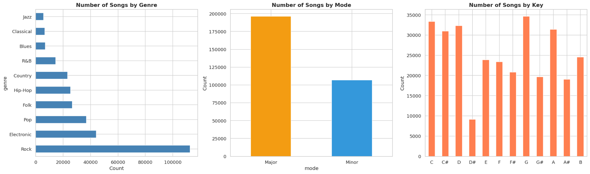
Observations:
- Genre: Rock dominates in volume (over 100,000 songs), followed by Electronic and Pop. Blues, Classical, and Jazz make up a very small proportion. However, higher quantity does not mean higher hit rate - this only reflects the data distribution, not the success rate.
- Mode: About two-thirds of songs use the Major scale (\~195,000) and one-third use Minor (\~110,000). Major scales typically convey a brighter, more uplifting feel - consistent with mainstream music preferences.
- Key: C, C#, G, and F# are the most popular keys (30,000–35,000 songs each). D# is the least popular (\~8,000 songs). The distribution is relatively even, with no single key holding absolute dominance.
4.3. Correlation Matrix Between Audio Features and Popularity
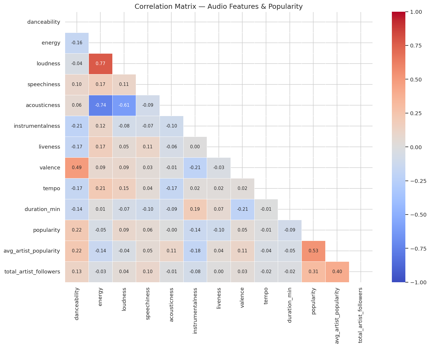
Observations:
- Strongest positive correlations with popularity: avg_artist_popularity (r \= 0.53) and total_artist_followers (r \= 0.31). Artist fame is the single strongest predictor of song success - far exceeding any individual audio feature.
- Top audio features with positive correlation: danceability (r \= 0.22) leads the pack, followed by loudness (r \= 0.09) and speechiness (r \= 0.06).
- Notable negative correlations: instrumentalness (r \= −0.14) and liveness (r \= −0.10) are the two audio features most negatively associated with popularity - songs without vocals and live-sounding recordings tend to be less popular.
- Between features themselves: energy and loudness are highly correlated (r \= 0.77), while energy and acousticness are strongly inversely correlated (r \= −0.74). These pairs carry significant overlapping information - an important consideration for any future predictive modeling.
- Near-zero correlations: acousticness (r \= −0.00), tempo (r \= −0.01), and duration_min (r \= −0.09) show virtually no linear relationship with popularity.
5. Do Artists Create Hits, Or Hits Create Artists?
Based on the correlation table, we can observe that the popularity of a song has the clearest relationship with the popularity of the artist who created it. In this section, we will explore this relationship in greater depth.
5.1. The Relationship Between Song Popularity and Artist Popularity
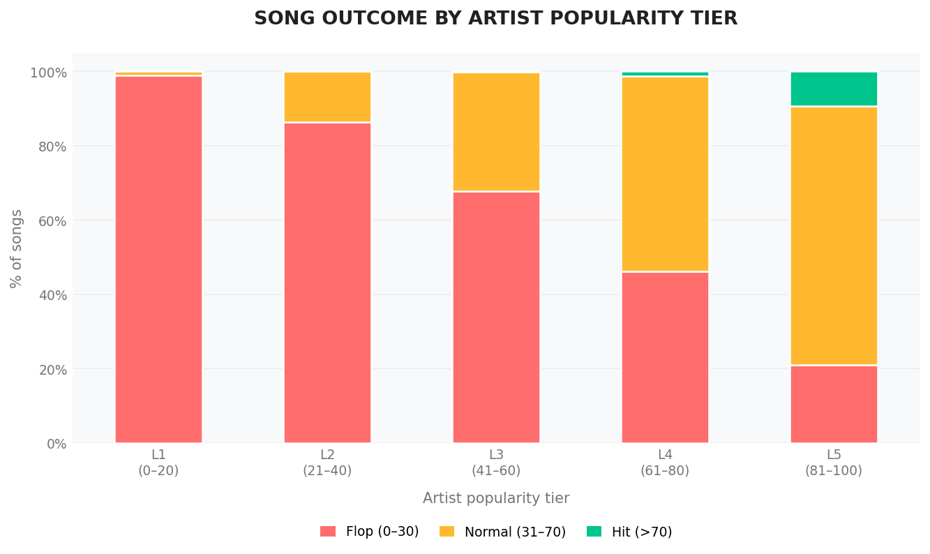
From the data above, we can see that most HIT songs come from artists who already have relatively high popularity, typically from 61 and above, with the majority concentrated in the 81–100 group. This suggests that an artist's reputation may play an important role in helping a song quickly reach a large audience. When an artist already has a substantial fan base, each of their new releases almost automatically has a "runway" for exposure and distribution.
However, the current data still cannot fully answer an important question: Do famous artists create HIT songs, or do HIT songs create famous artists - or both?
This relationship may be bidirectional, but determining the exact cause-and-effect relationship is beyond the scope of our analysis in this blog.
5.2. The Effect of Collaboration on Song Popularity
To further explore the influence of artists on the success of their songs, we decided to examine another aspect of the music industry: COLLABORATION.
Collaborations between artists have long been a familiar and exciting part of the music industry. For example, collaborations such as Son Tung M-TP and Snoop Dogg, or Rosé and Bruno Mars, often bring fresh musical experiences to audiences.
This leads to another question: Does collaboration between artists actually make a song more popular?
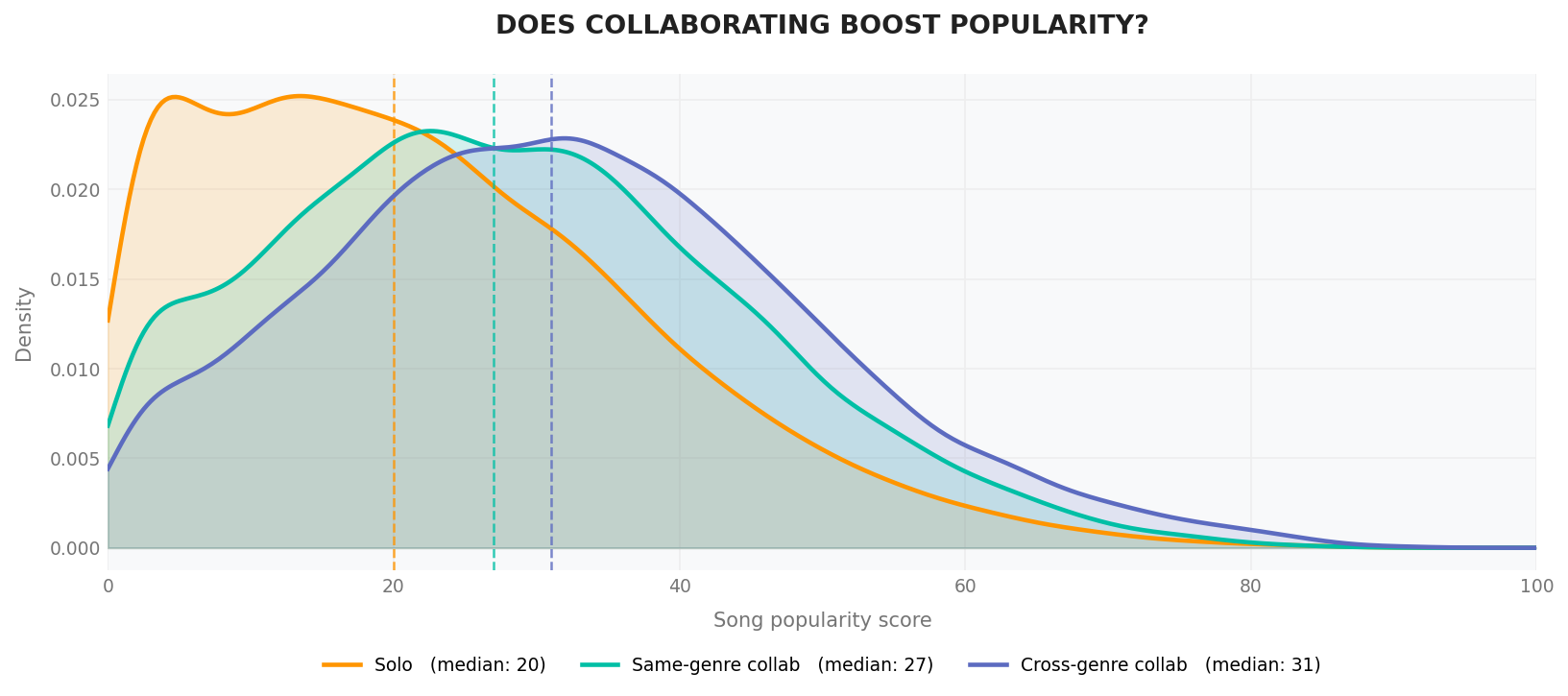
Our analysis shows that the distribution of popularity for collaborative songs is generally higher than that of solo songs. In particular, songs created by artists from different musical genres tend to have the highest popularity distribution, with a median of around 31. However, we cannot conclude whether collaboration itself makes songs more likely to become popular, or are the artists who collaborate already more famous to begin with?
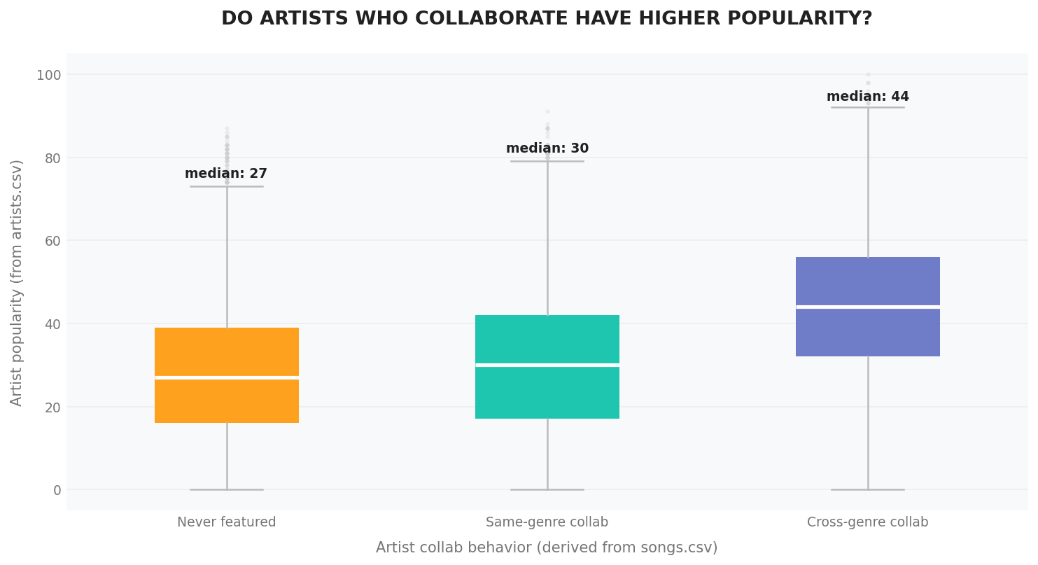
According to the chart, we can observe that artists who collaborate with others - especially those from different genres - tend to be more popular than artists who have never collaborated. This may indicate that more famous artists have more opportunities to collaborate, which in turn makes collaborative songs more likely to gain popularity.
5.3. The Career Age of Artists
The final question we explore in this section is whether an artist's career age is related to their ability to produce HIT songs. We measure an artist's career age by taking the year of their most recent song and subtracting the year of their first released song.
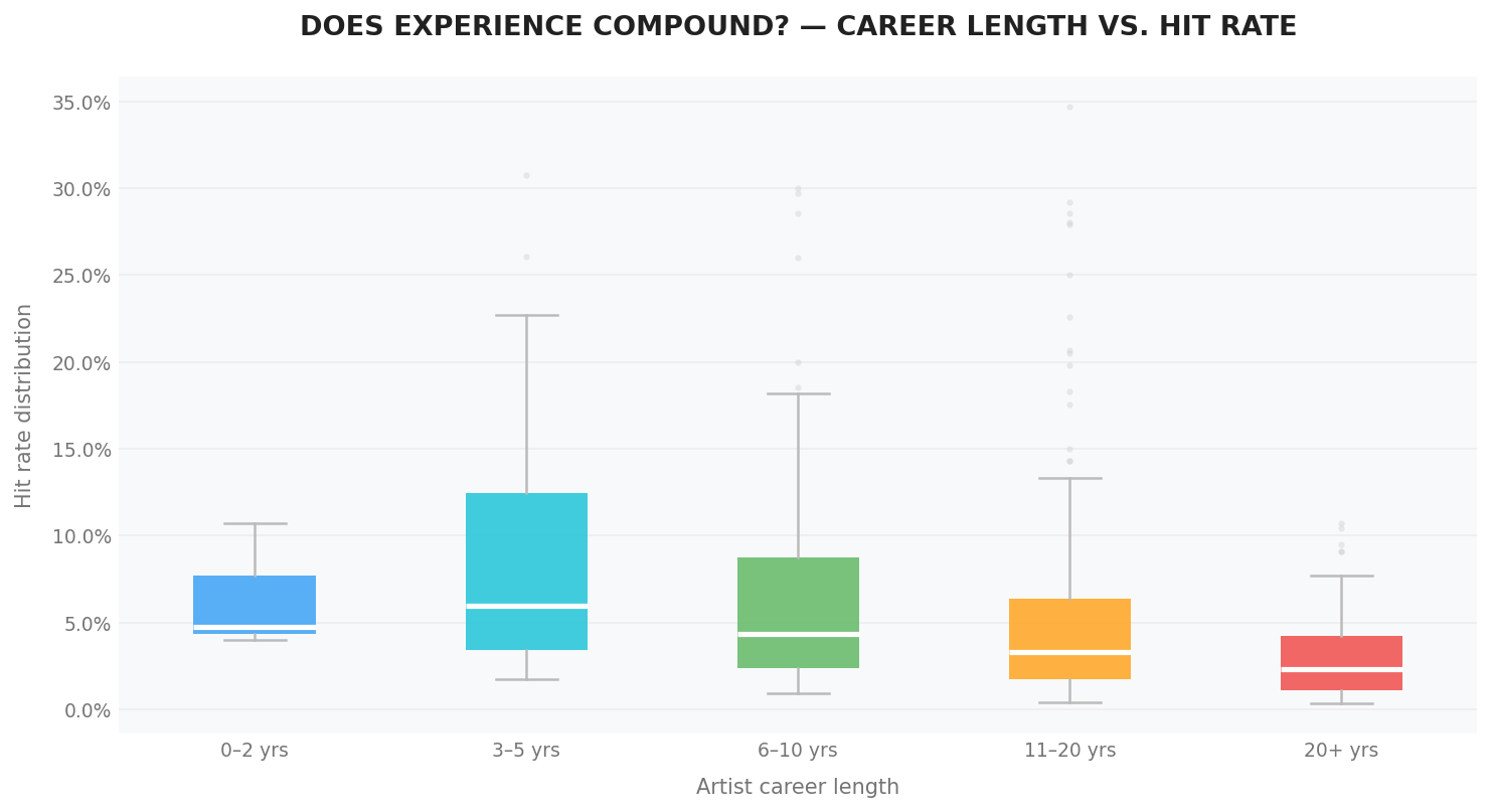
The data reveals a rather interesting observation. The median HIT rate increases slightly when moving from the group of artists with 0–2 years of activity to the group with 3–5 years, but then gradually decreases in groups with longer career spans.
This suggests that an artist's HIT rate tends to increase slightly during the early years of their career and reaches its highest level within the early stage (around 0–5 years). After that, the rate gradually declines over time, possibly because their music may no longer align as well with evolving public tastes and market trends.
Additionally, the data dispersion for artists with 3–5 years of career age is higher than in other groups. This may indicate that this period is a breakthrough stage for many artists, when some of them rise rapidly and become true HITmakers.
In summary, we can observe a relatively clear correlation between artists and the popularity of their songs, particularly in terms of the artist's own popularity. However, to confirm whether artists are truly a causal factor influencing song popularity, further research would be required (for example, through methods such as A/B testing).
6. The Battle Of The Genres
Have you ever wondered why the 'national anthems' that dominated the airwaves in the 2000s have now become a rarity on the charts? Is it truly our musical taste that has shifted, or are 'algorithms' and data silently redefining the very concept of a Hit? Let's revisit the past 25 years of music history through the lens of Data to see which 'empires' have fallen and who truly holds the crown of Popularity today.
6.1. Correlation Ratio between Genre and Popularity
The Correlation Ratio (denoted by the Greek letter η - Eta) is a statistical metric used to measure the strength of the relationship between a categorical variable (such as Genre) and a continuous numerical variable (such as Popularity).
The Core Concept: This algorithm operates by comparing the variance of the data in two distinct ways:
- Within-group variance: The dispersion of Popularity scores inside each specific genre.
- Between-group variance: The differences in the average Popularity scores between the different genres.
The Formula:
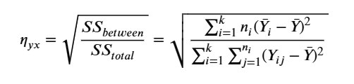
-
k: The total number of groups (musical genres). e.g., Pop, Rock, Jazz...
-
nᵢ: The number of songs within the $i^{th}$ genre.
-
ȳᵢ: The average Popularity score of the $i^{th}$ genre (e.g., the mean score specifically for the Rock genre).
-
ȳ: The overall mean Popularity score of all songs across the entire dataset.
-
yᵢⱼ: The Popularity score of the $j^{th}$ song within the $i^{th}$ genre.
Interpretation of η (ranging from 0 to 1):
- η \= 0: Genre has no correlation with popularity. The average scores for Rock, Pop, Blues, etc., are identical.
- η \= 1: Genre completely determines popularity. If you know a song is "Rock," you can predict its Popularity score with 100% accuracy.
- In Practice: In music datasets, η typically falls between 0.1 and 0.3. This indicates that while genre certainly has an influence, there are many other contributing factors such as the artist's brand, release timing, and marketing strategies that impact the final popularity score.
Implementation in Python
def calculate_correlation_ratio1(categories, measurements):
    fcat = categories.values
    fmeas = measurements.values
    y_avg_all = np.mean(fmeas)
    tmp_df = pd.DataFrame({'cat': fcat, 'meas': fmeas})
    group_stats = tmp_df.groupby('cat')['meas'].agg(['mean', 'count'])
    ss_between = np.sum(group_stats['count'] * (group_stats['mean'] - y_avg_all)**2)
    ss_total = np.sum((fmeas - y_avg_all)**2)
    eta = np.sqrt(ss_between / ss_total)
    return eta
After analyzing the correlations, the Correlation Ratio (η \= 0.2480) confirms that Genre falls within a range that significantly influences a song's success. Consequently, we will delve deeper into the specific impacts of genre on the music making process.
6.2. Popularity Distribution Across Genres
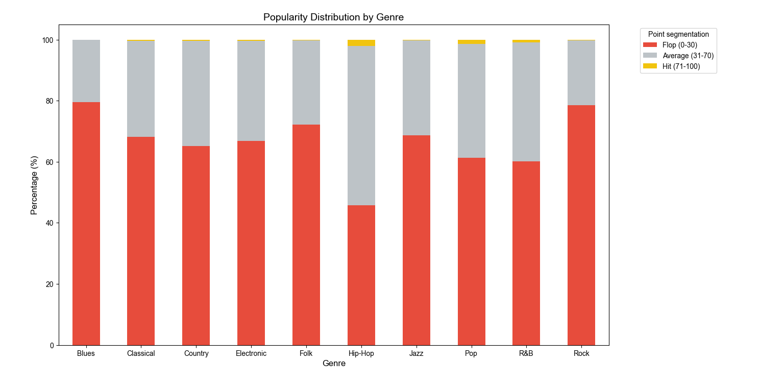
Hip-Hop Claims the Crown: While most other genres are "submerged" by a failure rate (Flop) ranging from 60% to nearly 80%, Hip-Hop stands alone as the only genre maintaining an outstanding proportion of Average and Hit tracks. With nearly 55% of its songs performing above the safety threshold, Hip-Hop proves itself not as a fleeting trend, but as a resilient "Hit-making machine."
The Decline of Blues and Rock: In stark contrast to that glory, Blues and Rock are navigating a period of profound challenges. The Flop rate (0-30 points) for these two genres is staggering approaching 80% leaving the Hit segment (represented in yellow) as thin as a thread.
The Safety Zone (Average): Genres like Pop and R\&B are successfully sustaining their presence with a significant volume of tracks in the intermediate zone, creating a stable foundation for the mainstream music market.
6.3. Popularity Dispersion
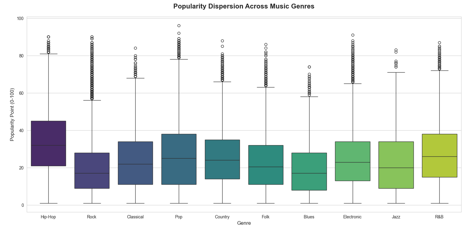
Hip-Hop: The "King" of the Common Ground: Hip-Hop holds the highest median value among all categories. This indicates that a randomly selected Hip-Hop track has a higher probability of becoming popular compared to any other genre.
Extreme Polarization in Pop & Rock: Although their "boxes" are situated in the lower range (indicating a high volume of "Flops"), these genres possess a dense and towering array of Outliers. This is the "all or nothing" group where a song either vanishes without a trace or skyrockets into a global mega hit.
Blues & Jazz: Lacking Momentum: These genres exhibit a narrow dispersion (IQR) and short upper whiskers. The data suggests that while their popularity is stable, they face significant hurdles in breaking through to reach a mainstream mass audience.
6.4. The Crown Exchange: The Great Migration of Hits
Hit Trends of the Top 5 Genres Over Time

The Fall of the "Rock Empire"
Starting at a towering peak of over 60% market share in 2000-01, Rock has undergone a continuous freefall, currently struggling to stay below 10%. This signifies the collapse of an era. Rock has lost its "monopoly" status, gradually giving way to genres that are catchier and better suited for the modern streaming era.
Hip-Hop & Pop: The Race for Global Dominance
- Hip-Hop (Yellow Line): This genre shows the most resilient and robust growth. Peaking in 2018-19, Hip-Hop accounted for nearly 50% of all hits in the market. Despite a slight dip in the final stages, it remains the most dominant force.
- Pop (Green Line): As Hip-Hop's most formidable rival, Pop maintains extremely stable performance within the 30-40% range. The intersection of Pop and Hip-Hop around 2022-23 suggests that listener tastes are reaching a balance between these two heavyweights.
The "Potential" Group (Electronic & R\&B)
Both genres have shown an upward trend over the last 2-3 years. Notably, Electronic is showing signs of recovery and renewed growth after a prolonged period of stagnation.
This chart serves as "smoking gun" evidence that music is never static. If the year 2000 was the stage for Rock, then 2025 is the playground of Hip-Hop and Pop. A perfect exchange of the crown has been completed over the course of more than two decades
7. When words speak
After exploring the diversity of music genres, a question remains: What truly makes a listener stay with a song? The answer lies in the lyrics. Lyrics are not just lifeless words; they are the emotional bridge between the artist and the audience. In this section, we use a "data lens" to deconstruct exactly how much content is "just right" and which specific keywords are truly dominating the global charts.
To measure this argument, we used correlation coefficients for verification. The results showed that word count significantly influences a song's chances of reaching the Top rankings.
The correlation formula we used:
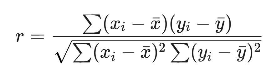
Where x is the number of words and y is the Popularity index.
7.1. Lyrics preprocessing
We processed the lyrics column in the dataset into two columns: the total number of words and the number of unique words in a song, for easier processing of WordCloud (in section 7.3). Then, we calculated the correlation between popularity and vocabulary, as well as the length of the lyrics:
df['word_count'] = df['lyrics'].apply(lambda x: len(str(x).split()))
df['unique_word_count'] = df['lyrics'].apply(lambda x: len(set(str(x).lower().split())))

# Tính Lexical Diversity (Độ đa dạng từ vựng)
df['lexical_diversity'] = df['unique_word_count'] / df['word_count']
df.loc[df['word_count'] == 0, 'lexical_diversity'] = 0

cols_to_check = ['popularity', 'word_count', 'unique_word_count', 'lexical_diversity']
correlation = df[cols_to_check].corr()
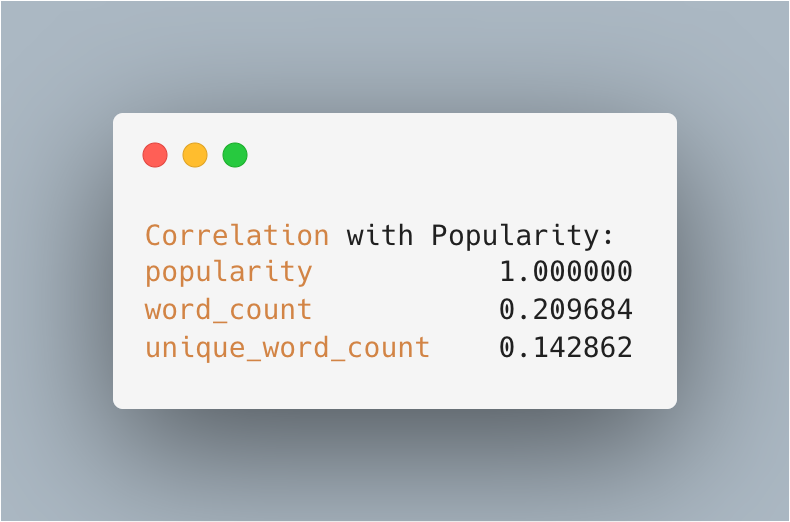
The results show that words correlated with popularity with r \= 0.209684 and r \= 0.142862, respectively, from the total number of words in the song and the list of unique words. Here we see that there is a basis for a song's popularity based on lyric length and word variety
7.2. The "Just Right" Zone: Why Lengthy or Minimalist Lyrics Rarely Hit the Charts.
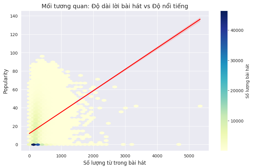
Our Hexbin density plot identifies a massive cluster (the brightest zone) between 200 and 500 words. This is the content "Sweet Spot." It proves that modern listeners prefer songs with enough lyrical substance to weave a narrative (Storytelling) without being overly verbose. Tracks outside this range (e.g., over 1000 words) show significantly lower popularity, suggesting that "word stuffing" is rarely a winning strategy for achieving mainstream success.
7.3. The Hit Dictionary: Keywords that Haunt the Listener's Mind.
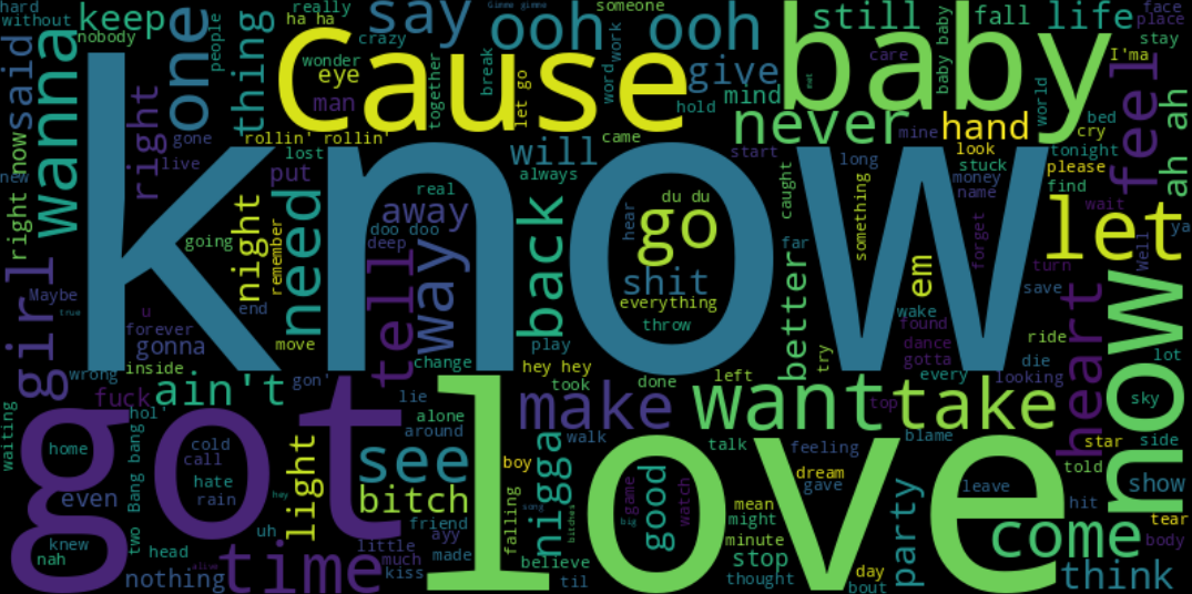
The Word Cloud deconstructs the soul of the most successful tracks. The prominent presence of terms like "Love", "Baby", "Know", and "Feel" reveals two dominant themes: Emotional Connection and Self-Assertion. Listeners turn to music to feel understood (through "Love" and "Time") but also to find personal strength (through powerful verbs like "Know", "Will", and "Can"). These are the "universal" keywords that allow a song to resonate deeply with millions of people.
In conclusion, successful lyrics aren't just about what you say, but also how much you say. Our data clearly indicates that a well-balanced content structure (300-500 words), combined with messages centered on love and empowerment, is the "key" to unlocking high popularity. Lyrics are where art meets mathematics—where the frequency of words translates into the most powerful emotional vibrations.
8. CONCLUSION - IS THERE A FORMULA FOR A HIT?
After analyzing a massive dataset of songs from 2000–2025 on Spotify, the short answer is: there are clear patterns, but no "magical formula."
The data shows that hits are not random - they tend to share certain common characteristics. Successful songs are generally more danceable (high danceability), louder (high loudness), less purely instrumental (low instrumentalness), and carry a polished studio-recorded sound rather than a live performance feel (low liveness). However, these audio features individually show only weak to moderate correlations with popularity - the strongest being danceability at r \= 0.22.
The most influential factor turns out to lie not in the song itself, but in the artist behind it. With r \= 0.53, artist popularity is the single strongest predictor of a song's success - far surpassing all audio features combined. Already-famous artists have a built-in "runway" that allows each new release to quickly reach audiences. Additionally, collaborations between artists - especially cross-genre ones - tend to achieve higher popularity than solo tracks. And interestingly, the 3–5 year career mark appears to be the golden window for producing hits, before success rates gradually decline over time.
In terms of genre, Hip-Hop has proven to be the most consistent hit-making "machine" over the past two decades, while Rock - which once dominated with over 60% of hit market share in 2000 - now accounts for less than 10%. Pop has maintained steady performance, and the growing crossover between Pop and Hip-Hop in recent years clearly reflects shifting listener preferences.
In summary, success in music is multifactorial. Audio features paint a general "portrait" of a hit, but they alone cannot guarantee success. Artist reputation, genre trends, release timing, marketing strategy, and collaborations all play critical roles. And with only 0.59% of songs crossing the hit threshold, there is clearly no shortcut to the top.
Data can reveal the patterns behind success, but the magic of music always leaves room for surprise - and perhaps that is exactly what makes music endlessly captivating.
Chưa có bình luận nào. Hãy là người đầu tiên!