Introduction
Linear Regression is one of the most fundamental and widely used techniques in the field of Machine Learning and Data Analysis. It provides a simple yet powerful framework for modeling the relationship between input variables and an output variable, allowing us to understand and predict real-world phenomena. Despite its simplicity, Linear Regression serves as the foundation for many advanced predictive and statistical models used in modern applications.
Linear Regression is extensively applied across a variety of domains, including:
- Price Forecasting: Used to predict values such as house prices, stock prices, or fuel prices based on
influential factors like location, size, quality, and supply-demand dynamics. - Score Prediction: Applied in education to estimate student performance based on variables such as
study time, effort, skill level, and teacher qualifications. - Product Forecasting: Used in manufacturing to estimate production output depending on time,
machine capacity, raw material availability, and labor resources. - Time Series Analysis: Utilized to predict future trends, patterns, and seasonal cycles in various
areas such as real estate, climate, and industrial productivity.
The key strength of Linear Regression lies in its interpretability and efficiency. It helps decision-makers understand how changes in one or more variables affect an outcome, thereby providing valuable insights for forecasting, planning, and optimization. As one of the earliest and most essential techniques in data science, Linear Regression continues to play a crucial role in both academic research and practical applications across industries.
1. Model
Linear Regression is a supervised learning algorithm used to model the relationship between a dependent variable (target) and one or more independent variables (features). Its main objective is to find the best-fitting linear relationship that explains how changes in the input variables affect the output variable. One of the popular ways to estimate the coefficients is to use the Ordinary Least Squares (OLS) method, where we need to minimize the sum of squared errors.
From a practical perspective, Linear Regression provides both prediction and interpretation:
- It predicts future outcomes based on historical data.
- It quantifies relationships — showing how much each feature contributes to the output.
- It forms the foundation for more complex models in machine learning, such as logistic regression, ridge regression, and neural networks.
In short, Linear Regression is not only a predictive tool but also an explanatory one, offering clear insight into how variables interact in a linear manner.
1.1. Model Representation
The hypothesis function (or prediction function) of a linear regression model is expressed as:
$$ \hat{y} = w_0 + w_1x_1 + w_2x_2 + \dots + w_nx_n $$
where:
- $\hat{y}$ is the predicted output (target value),
- $x_i$ represents the $i$-th feature,
- $w_i$ denotes the corresponding weight (coefficient),
- $w_0$ is the bias (intercept) term.
In vectorized form, the equation can be written compactly as:
$$ \hat{y} = \mathbf{w}^\top \mathbf{x} + b $$
where $\mathbf{w} = [w_1, w_2, \dots, w_n]^\top$ and $\mathbf{x} = [x_1, x_2, \dots, x_n]^\top$.
1.2. Training Procedure
The training process of Linear Regression aims to find the optimal parameters (weight vector $\mathbf{w}$ and bias $b$) that minimize the loss function, typically the Mean Squared Error (MSE). This section outlines the step-by-step training procedure.
Step 1: Select a Training Sample
Choose a random data sample $(x_1, x_2, x_3, y)$ from the training dataset,
where $x_1, x_2, x_3$ represent the input features and $y$ is the true output (label).
$$ (x_1, x_2, x_3) \in \mathbb{R}^3, \quad y \in \mathbb{R} $$
The goal of the model is to predict an output $\hat{y}$ that approximates the true label $y$.
Step 2: Compute the Predicted Output
Using the current values of weights and bias, compute the predicted output $\hat{y}$ for the selected sample:
$$ \hat{y} = w_1x_1 + w_2x_2 + w_3x_3 + b $$
where:
- $w_i$ denotes the weight associated with feature $x_i$,
- $b$ is the bias term that shifts the regression line or hyperplane.
This step represents the forward pass of the model.
Step 3: Compute the Loss Function
To measure how far the predicted value $\hat{y}$ is from the true value $y$,
we use the Mean Squared Error (MSE) loss function.
For a single data sample, the loss is given by:
$$
L = (\hat{y} - y)^2
$$
This value represents the squared difference between the predicted and true outputs. The higher the value of $L$, the worse the prediction.
Step 4: Compute the Derivatives (Gradients)
To minimize the loss, we need to determine how each parameter ($w_1, w_2, w_3, b$) affects the loss function. This is achieved by calculating the partial derivatives (gradients) of $L$ with respect to each parameter:
$$ \frac{\partial L}{\partial w_1} = 2x_1(\hat{y} - y), \quad \frac{\partial L}{\partial w_2} = 2x_2(\hat{y} - y), \quad \frac{\partial L}{\partial w_3} = 2x_3(\hat{y} - y) $$
$$ \frac{\partial L}{\partial b} = 2(\hat{y} - y) $$
The gradient indicates both:
- The direction in which the loss increases, and
- The magnitude of change in the loss with respect to each parameter.
By following the opposite direction of the gradient, the model reduces the loss function.
Step 5: Update the Parameters
The parameters are updated using the Gradient Descent optimization algorithm. Each parameter moves in the direction opposite to its gradient, scaled by the learning rate $\eta$ (eta):
$$ w_1 = w_1 - \eta \frac{\partial L}{\partial w_1}, \quad w_2 = w_2 - \eta \frac{\partial L}{\partial w_2}, \quad w_3 = w_3 - \eta \frac{\partial L}{\partial w_3}, \quad b = b - \eta \frac{\partial L}{\partial b} $$
where:
- $\eta$ is the learning rate, a hyperparameter that controls how large each update step is.
- A smaller $\eta$ leads to slower but more stable convergence.
- A larger $\eta$ may speed up training but risks overshooting the minimum.
Summary
The training loop iteratively repeats the following steps for many epochs until convergence:
- Select a data sample or batch.
- Compute prediction $\hat{y}$.
- Evaluate the loss $L$.
- Compute gradients of $L$ with respect to parameters.
- Update parameters using gradient descent.
Over multiple iterations, the parameters $(w_1, w_2, w_3, b)$ gradually adjust to minimize the overall loss,
leading to a model that best fits the training data.
1.3. Training Strategy
1.3.1. Mini-batch Training
Mini-batch training provides a balance between stochastic gradient descent (SGD) (where $m=1$) and batch gradient descent (where $m=N$).
In stochastic training, updates are frequent and fast but noisy.
In batch training, updates are smooth and stable but computationally slow.
Mini-batch training offers the best of both worlds.
Definition and Process
In mini-batch training, at each iteration, a random subset of $m$ samples (called a mini-batch) is selected from the training dataset. The dataset is usually shuffled at the beginning of each epoch to ensure that the model does not learn in a fixed order.
The training process for one mini-batch can be summarized as follows:
-
Forward Pass:
Compute the predicted outputs $\hat{y}_i$ for all $m$ samples in the mini-batch:
$$ \hat{y}_i = w^T x_i + b $$ -
Compute Loss:
Calculate the average loss across the mini-batch using Mean Squared Error (MSE):
$$ L = \frac{1}{m} \sum_{i=1}^{m} (\hat{y}_i - y_i)^2 $$ -
Compute Gradient:
Derive the gradient of the loss function with respect to model parameters:
$$ \frac{\partial L}{\partial w} = \frac{1}{m} \sum_{i=1}^{m} 2x_i(\hat{y}_i - y_i) \quad \text{and} \quad \frac{\partial L}{\partial b} = \frac{1}{m} \sum_{i=1}^{m} 2(\hat{y}_i - y_i) $$ -
Update Parameters:
Update model weights and bias using gradient descent:
$$ w := w - \eta \frac{\partial L}{\partial w}, \qquad b := b - \eta \frac{\partial L}{\partial b} $$
Example
When training with a mini-batch size of $m=2$, the model starts with initial parameters $w = -0.34$ and $b = 0.04$, producing an initial loss of $L = 91.83$. After one update step, the parameters become $w = 0.761$ and $b = 0.227$. After $30$ iterations, the loss decreases significantly, demonstrating the efficiency of mini-batch training in improving model performance while maintaining stability.
Advantages and Disadvantages
Advantages:
- Reduces the variance of gradient estimates compared to stochastic training.
- Achieves faster convergence than full batch gradient descent for large datasets.
- Provides a good trade-off between computation time and convergence stability.
Disadvantages:
- Requires careful tuning of the mini-batch size $m$.
- Too small $m$ leads to noisy gradients; too large $m$ reduces computational efficiency.
Practical Notes
- Common mini-batch sizes typically range from $m = 32$ to $256$,
depending on dataset size and hardware capacity. - Compared to stochastic gradient descent, mini-batch updates exhibit less oscillation
and provide smoother learning curves. - Shuffling data before each epoch ensures randomness and avoids bias from data ordering.
1.3.2. Batch Training
Batch training is a training strategy in which the model uses the entire dataset ($m = N$) to compute the loss and gradients during each update step. This approach ensures accurate gradient computation across all training samples
but requires higher computational cost.
Training Process
The batch training process follows the same procedure as mini-batch training, except that the loss and gradients are averaged over the entire dataset of size $N$:
-
Forward Pass:
$$ \hat{y}_i = w^T x_i + b $$ -
Compute Loss:
$$ L = \frac{1}{N} \sum_{i=1}^{N} (\hat{y}_i - y_i)^2 $$ -
Compute Gradient:
$$ \frac{\partial L}{\partial w} = \frac{1}{N} \sum_{i=1}^{N} 2x_i(\hat{y}_i - y_i), \qquad \frac{\partial L}{\partial b} = \frac{1}{N} \sum_{i=1}^{N} 2(\hat{y}_i - y_i) $$ -
Update Parameters:
$$ w := w - \eta \frac{\partial L}{\partial w}, \qquad b := b - \eta \frac{\partial L}{\partial b} $$
Example
When using full batch training with $N = 4$ samples,
the initial loss is $L = 72.37$. After one update, the parameters become $w = 0.54$ and $b = 0.205$. After $30$ iterations, the model converges rapidly for small datasets, showing the stability and accuracy of batch training when data volume is limited.
Advantages and Disadvantages
Advantages:
- Produces exact gradient estimates by computing over all samples.
- Offers smooth and stable convergence with minimal noise.
- Suitable for small or moderate-sized datasets.
Disadvantages:
- Slow for large datasets because it requires processing the entire data before each update.
- High memory usage since all data must fit into memory.
- Less efficient when working with streaming or continuously updating datasets.
Comparison and Practical Notes
Empirical comparisons of losses and parameter updates show that batch training
achieves the most stable convergence patterns but with slower training speed compared
to mini-batch and stochastic methods.
Therefore, batch training is best suited for small datasets or when computational resources are sufficient.
1.4. Code Implementation
1.4.1. Gradient Descent Pipeline
-
Initialize $(\boldsymbol{\theta})$
-
Take all ( N ) samples
-
Compute $$ \hat{\mathbf{y}} = \mathbf{X} \boldsymbol{\theta} $$
-
Compute loss $$ \frac{1}{N} (\hat{\mathbf{y}} - \mathbf{y})^T (\hat{\mathbf{y}} - \mathbf{y}) $$
-
Compute gradient $$ \nabla_{\boldsymbol{\theta}} L = \frac{1}{N} \mathbf{X}^T [2 (\hat{\mathbf{y}} - \mathbf{y})] $$
-
Update $$ \boldsymbol{\theta} = \boldsymbol{\theta} - \eta \nabla_{\boldsymbol{\theta}} L $$
1.4.2. Version 1: 1-Sample
In the single-sample version, gradient descent is applied one sample at a time (stochastic gradient descent). Steps for a single sample are as follows:
For a sample $\mathbf{x}_i$ (augmented with 1 for bias) and $y_i$:
- Compute $\hat{y}_i = \boldsymbol{\theta}^T \mathbf{x}_i$
- Loss $L = (\hat{y}_i - y_i)^2$
- Gradient $\nabla_{\boldsymbol{\theta}} L = 2 (\hat{y}_i - y_i) \mathbf{x}_i$
- Update $\boldsymbol{\theta} = \boldsymbol{\theta} - \eta \nabla_{\boldsymbol{\theta}} L$
Example in Python (using NumPy for vector operations):
import numpy as np

# Single sample example
X_i = np.array([1, 3])  # [bias, experience]
y_i = 60
theta = np.array([10, 3])  # [b, w]
eta = 0.001

y_hat_i = np.dot(theta, X_i)
loss = (y_hat_i - y_i)**2
grad = 2 * (y_hat_i - y_i) * X_i
theta = theta - eta * grad
print(theta)
This updates parameters based on one sample per iteration.
1.4.3. Version 2: N-Samples
In the N-samples version (batch gradient descent), all samples are used to compute the average gradient.
For matrix $\mathbf{X}$ (N × (features + 1)) and vector $\mathbf{y}$ (N × 1):
- Compute $\hat{\mathbf{y}} = \mathbf{X} \boldsymbol{\theta}$
- Loss $L = \frac{1}{N} \| \hat{\mathbf{y}} - \mathbf{y} \|^2$
- Gradient $\nabla_{\boldsymbol{\theta}} L = \frac{2}{N} \mathbf{X}^T (\hat{\mathbf{y}} - \mathbf{y})$
- Update $\boldsymbol{\theta} = \boldsymbol{\theta} - \eta \nabla_{\boldsymbol{\theta}} L$
Example in Python (using NumPy):
import numpy as np

# N-samples example
X = np.array([[1, 3], [1, 4], [1, 5], [1, 6]])  # Bias + experience
y = np.array([60, 55, 66, 93])
theta = np.array([10, 3])  # [b, w]
eta = 0.001
N = len(y)

y_hat = np.dot(X, theta)
loss = (1/N) * np.sum((y_hat - y)**2)
grad = (2/N) * np.dot(X.T, (y_hat - y))
theta = theta - eta * grad
print(theta)
This computes the gradient over the entire dataset for more stable updates.
1.4.4. Compare Performance
The vectorized version using N-samples (batch gradient descent) is generally more efficient than the 1-sample version (stochastic gradient descent) for several reasons. In terms of computational performance, vectorized operations in libraries like NumPy leverage optimized matrix multiplications, which are faster than looping over individual samples, especially for large datasets. This leads to better utilization of hardware resources, such as vectorized instructions in CPUs or GPUs.
The 1-sample version can converge faster in terms of epochs due to more frequent updates but may oscillate around the minimum, requiring careful tuning of the learning rate. In contrast, the N-samples version provides smoother convergence as it averages gradients, reducing variance, but each iteration is computationally more expensive.
For example, on a dataset with thousands of samples, the vectorized batch approach can be 10-100x faster per epoch due to parallelization. However, for very large datasets that don't fit in memory, mini-batch versions (a compromise) are often used. In practice, the vectorized implementation scales better and is easier to maintain as the number of features increases.
2. Loss Function
2.1. Conditions for Loss Functions
In machine learning, a loss function measures the discrepancy between the predicted output $\hat{y}$ and the true target $y$. For a loss function to be mathematically suitable for optimization, it must satisfy certain conditions that ensure stable and efficient learning.
Two of the most important conditions are Continuity and Differentiability.
2.1.1. Continuity
Definition
A function $f(x)$ is said to be continuous at a point $x = a$ if and only if the following three conditions are satisfied:
- $f(a)$ is defined.
- The limit $\displaystyle \lim_{x \to a} f(x)$ exists.
- The limit equals the function value at that point:
$$ \lim_{x \to a} f(x) = f(a) $$
If any of these conditions fails, the function is said to be discontinuous at that point.
Continuity means that the function has no sudden jumps or breaks — in other words, you can draw its graph without lifting your pen from the paper. For loss functions, continuity ensures that small changes in model parameters produce small, predictable changes in the loss value. This stability is essential for numerical optimization methods such as Gradient Descent.
Examples of Continuity
Example 1: Continuous Function
Consider the polynomial function:
$$
f(x) = x^3 - 2x + 1
$$
Polynomial functions are continuous for all real numbers because they are composed only of basic arithmetic operations.
Such functions are smooth and ideal for optimization.
Example 2: Continuous but Non-Differentiable Function}
The function:
$$
f(x) = |x| \quad \text{or more generally} \quad f(x) = x^{1/3}
$$
is continuous everywhere but not differentiable at $x = 0$.
The graph of $|x|$ has a sharp corner at the origin, meaning the slope (derivative) is not defined at that point.
This type of function is common in loss functions such as Mean Absolute Error (MAE)}, which is continuous but non-differentiable at zero.
Example 3: Discontinuous Function
A function is discontinuous if it has a break, hole, or jump at some point.
For instance:
$$
f(x) =
\begin{cases}
3x^2 - 2, & x < 1 \\
2x - 1, & x > 1
\end{cases}
\quad \text{or} \quad f(x) = \frac{1}{x}
$$
Both are discontinuous — the first due to a jump at $x = 1$, and the second because it is undefined at $x = 0$.
Discontinuous loss functions are not suitable} for gradient-based optimization since the derivative cannot be computed reliably.
| Function Type | Continuous | Differentiable | Example |
|---|---|---|---|
| Continuous Function | Yes | Yes | $x^3 - 2x + 1$ |
| Continuous Non-Differentiable | Yes | No (at some points) | $|x|$, $x^{1/3}$ |
| Discontinuous Function | No | No | $\frac{1}{x}$, $\frac{3x^2 - 2}{2x - 1}$ |
Table: Examples of function types based on continuity and differentiability.
2.1.2. Differentiability
Definition
Let $f(x)$ be a function.
The derivative of $f$ at a point $x$ is defined as:
$$ f'(x) = \lim_{h \to 0} \frac{f(x + h) - f(x)}{h} $$
A function $f$ is said to be differentiable at $x = a$ if $f'(a)$ exists.
If $f'(x)$ exists for all $x$ in a region $S$, then $f$ is said to be differentiable on $S$.
A differentiable function is one that is both continuous and smooth (has a well-defined slope everywhere).
Differentiability ensures that we can compute a tangent (slope) to the function at any point.
This property is crucial for optimization algorithms such as Gradient Descent, which rely on the derivative of the loss function to update parameters in the direction that minimizes the loss.
Properties and Notes
- Every differentiable function is continuous, but not every continuous function is differentiable.
- Differentiability implies local linearity: near any point, the function behaves like a straight line.
- Loss functions that are differentiable allow smooth parameter updates, leading to faster convergence.
Examples
Example 1: Differentiable Function
$$
f(x) = x^2 \quad \Rightarrow \quad f'(x) = 2x
$$
This function is smooth and differentiable everywhere, making it ideal for use in loss functions such as Mean Squared Error (MSE).
Example 2: Non-Differentiable Function
$$
f(x) = |x| \quad \Rightarrow \quad
f'(x) =
\begin{cases}
1, & x > 0 \\
-1, & x < 0
\end{cases}
$$
At $x = 0$, the derivative does not exist because the left and right limits are not equal. This demonstrates that even continuous functions can fail to be differentiable.
Importance in Machine Learning:
Differentiability is required to compute gradients for model optimization.
A differentiable loss function ensures that the learning process can adjust parameters smoothly and effectively using gradient-based algorithms.
2.2. Three Fundamental Loss Functions
In machine learning, a loss function quantifies the difference between the predicted value $\hat{y}$ and the true target value $y$. It measures how well a model performs on a given dataset and provides a feedback signal for optimization algorithms such as Gradient Descent. A good loss function should be continuous, differentiable (or sub-differentiable), and sensitive to prediction errors.
This section introduces three fundamental loss functions commonly used in regression tasks:
Mean Absolute Error (MAE), Mean Squared Error (MSE), and Huber Loss.
2.2.1. Mean Absolute Error (MAE)
The Mean Absolute Error measures the average of the absolute differences between predicted and actual values:
$$ L_{\text{MAE}} = \frac{1}{N} \sum_{i=1}^{N} |y_i - \hat{y}_i| $$
Characteristics
- Continuous but not differentiable at zero.
- Less sensitive to outliers than MSE.
- Produces a constant gradient magnitude (except at zero).
Gradient Derivation
For a single data point:
$$
L = |\hat{y} - y|
$$
The partial derivatives with respect to model parameters $(w, b)$ are:
$$
\frac{\partial L}{\partial w} = x \cdot \frac{(\hat{y} - y)}{|\hat{y} - y|}, \qquad
\frac{\partial L}{\partial b} = \frac{(\hat{y} - y)}{|\hat{y} - y|}
$$
At $\hat{y} = y$, the gradient is undefined but can be approximated as zero using subgradient methods.
Parameter Update Rule
$$ w = w - \eta \frac{\partial L}{\partial w}, \qquad b = b - \eta \frac{\partial L}{\partial b} $$
Advantages and Disadvantages
- Advantages: Robust to outliers; represents median-like behavior.
- Disadvantages: Non-differentiability at zero; slower convergence than MSE.
2.2.1. Mean Squared Error (MSE)}
The Mean Squared Error} computes the average of squared differences between predicted and true values:
$$ L_{\text{MSE}} = \frac{1}{N} \sum_{i=1}^{N} (y_i - \hat{y}_i)^2 $$
Characteristics
- Continuous and differentiable everywhere.
- Penalizes large errors more strongly due to the square term.
- Widely used because of its smoothness and convenient mathematical properties.
Gradient Derivation
For a single data point:
$$
L = (\hat{y} - y)^2
$$
The partial derivatives are:
$$
\frac{\partial L}{\partial w} = 2x(\hat{y} - y), \qquad
\frac{\partial L}{\partial b} = 2(\hat{y} - y)
$$
Parameter Update Rule
$$ w = w - \eta \frac{\partial L}{\partial w}, \qquad b = b - \eta \frac{\partial L}{\partial b} $$
Advantages and Disadvantages
- Advantages: Smooth, differentiable, and suitable for gradient-based optimization.
- Disadvantages: Very sensitive to outliers; large errors dominate the loss.
2.2.2. Huber Loss
The Huber Loss combines the strengths of both MAE and MSE.
It behaves quadratically for small errors and linearly for large errors, offering robustness to outliers while maintaining differentiability.
$$
L_{\delta}(y, \hat{y}) =
\begin{cases}
\frac{1}{2}(y - \hat{y})^2, & \text{if } |y - \hat{y}| \leq \delta \\
\delta(|y - \hat{y}| - \frac{1}{2}\delta), & \text{otherwise}
\end{cases}
$$
where $\delta$ is a threshold parameter determining the transition point between MSE and MAE regions.
Gradient Derivation
$$
\frac{\partial L}{\partial w} =
\begin{cases}
x(\hat{y} - y), & \text{if } |\hat{y} - y| \leq \delta \\
\delta x \frac{(\hat{y} - y)}{|\hat{y} - y|}, & \text{otherwise}
\end{cases}
$$
$$
\frac{\partial L}{\partial b} =
\begin{cases}
(\hat{y} - y), & \text{if } |\hat{y} - y| \leq \delta \\
\delta \frac{(\hat{y} - y)}{|\hat{y} - y|}, & \text{otherwise}
\end{cases}
$$
Advantages and Disadvantages
- Advantages: Differentiable everywhere; balances sensitivity to outliers and smooth optimization.
- Disadvantages: Requires tuning of $\delta$; performance depends on the data distribution.
Comparison Summary
| Property | MSE | MAE | Huber |
|---|---|---|---|
| Continuity | Yes | Yes | Yes |
| Differentiability | Yes | No (at 0) | Yes |
| Outlier Sensitivity | High | Low | Medium |
| Penalty Type | Quadratic | Linear | Hybrid |
| Optimization Stability | High | Moderate | High |
Table: Comparison among MSE, MAE, and Huber Loss functions.
2.3. Regularization
In regression models, minimizing the loss function alone often leads to overfitting,
where the model learns noise or random fluctuations in the training data rather than the true underlying patterns.
Regularization is a technique that introduces a penalty term into the loss function to constrain the model parameters,
preventing them from becoming excessively large and thus improving generalization on unseen data.
Motivation
When training a linear regression model:
$$
\hat{y} = w_1x_1 + w_2x_2 + \dots + w_nx_n + b
$$
the standard Mean Squared Error (MSE) loss is:
$$
L = \frac{1}{N}\sum_{i=1}^{N}(y_i - \hat{y}_i)^2
$$
If the model fits the training data too closely, the learned weights $(w_1, w_2, \dots, w_n)$ may grow very large in magnitude, leading to poor performance on new data (high variance). Regularization mitigates this by adding a penalty term that discourages large weights.
General Formulation
A regularized loss function can be written as:
$$
L_{\text{reg}} = L + \lambda \Omega(\mathbf{w})
$$
where:
- $L$ is the original loss (e.g., MSE or MAE),
- $\Omega(\mathbf{w})$ is the regularization term,
- $\lambda > 0$ is the regularization coefficient controlling the penalty strength.
The parameter $\lambda$ determines the balance between minimizing the training error and keeping model weights small:
- Small $\lambda$ $\Rightarrow$ weak regularization, potentially leading to overfitting.
- Large $\lambda$ $\Rightarrow$ strong regularization, possibly leading to underfitting.
Types of Regularization
Two common types of regularization are L2 Regularization (Ridge) and L1 Regularization (Lasso).
(a) L2 Regularization (Ridge Regression)
L2 regularization adds the squared magnitude of weights as a penalty term:
$$
L_{\text{Ridge}} = \frac{1}{N}\sum_{i=1}^{N}(y_i - \hat{y}_i)^2 + \lambda \sum_{j=1}^{n} w_j^2
$$
The gradient of the loss function becomes:
$$
\frac{\partial L_{\text{Ridge}}}{\partial w_j} = -2x_j(y - \hat{y}) + 2\lambda w_j
$$
L2 regularization encourages weights to remain small but not exactly zero, resulting in smooth solutions and numerical stability.
(b) L1 Regularization (Lasso Regression)}
L1 regularization penalizes the absolute values of the weights:
$$
L_{\text{Lasso}} = \frac{1}{N}\sum_{i=1}^{N}(y_i - \hat{y}_i)^2 + \lambda \sum_{j=1}^{n} |w_j|
$$
The gradient (subgradient) is:
$$
\frac{\partial L_{\text{Lasso}}}{\partial w_j} = -2x_j(y - \hat{y}) + \lambda \, \text{sign}(w_j)
$$
L1 regularization can drive some weights exactly to zero, leading to sparse models, which is useful for feature selection.
Comparison Between L1 and L2 Regularization
| Property | L1 Regularization (Lasso) | L2 Regularization (Ridge) |
|---|---|---|
| Weight shrinkage | May become exactly zero | Shrinks toward zero but never exactly zero |
| Model sparsity | Produces sparse weights (feature selection) | Keeps all features (no sparsity) |
| Optimization surface | Diamond-shaped constraint | Circular/elliptical constraint |
| Computational stability | May be less stable | More stable and smooth |
Table: Comparison between L1 and L2 regularization techniques.
Effect on Optimization Landscape
Without regularization, the loss surface may have narrow valleys and sharp minima, leading to unstable gradient updates.
Regularization smooths the loss surface, producing broader and more stable minima, which improves convergence and generalization.
Example: Regularized Linear Regression
For a linear regression model with two features $(x_1, x_2)$:
$$
\hat{y} = w_1x_1 + w_2x_2 + b
$$
the regularized loss with L2 penalty is:
$$
L = (\hat{y} - y)^2 + \lambda (w_1^2 + w_2^2)
$$
The corresponding gradients are:
$$
\frac{\partial L}{\partial w_1} = 2x_1(\hat{y} - y) + 2\lambda w_1, \qquad
\frac{\partial L}{\partial w_2} = 2x_2(\hat{y} - y) + 2\lambda w_2
$$
$$
\frac{\partial L}{\partial b} = 2(\hat{y} - y)
$$
Parameter updates follow:
$$
w_j := w_j - \eta \frac{\partial L}{\partial w_j}, \qquad
b := b - \eta \frac{\partial L}{\partial b}
$$
This ensures that both the prediction error and the weight magnitudes are minimized simultaneously.
3. Data
3.1. Data Normalization
Data Normalization is a preprocessing technique that scales the values of features to a common range. It is essential for improving the stability, convergence speed, and accuracy of machine learning models, especially those that rely on gradient-based optimization methods such as linear regression, logistic regression, or neural networks.
Unnormalized Data Example
For unnormalized features, the training process uses a small learning rate $\eta = 10^{-5}$ to prevent divergence.
$$ \hat{y} = w_1 x_{\text{1}} + w_2 x_{\text{2}} + w_3 x_{\text{3}} + b $$
During training:
$$
w_j := w_j - \eta \frac{\partial L}{\partial w_j}, \qquad
b := b - \eta \frac{\partial L}{\partial b}
$$
However, because feature magnitudes differ significantly, gradients across parameters vary widely, making convergence extremely slow and unstable.
Normalized Data Example
After normalization, features are transformed to a comparable scale using methods such as:
$$
x' = \frac{x - \mu_x}{x_{\max} - x_{\min}}
\quad \text{(Min-Max Normalization)}
$$
or
$$
x' = \frac{x - \mu_x}{\sigma_x}
\quad \text{(Z-score Normalization)}
$$
Where:
- $\mu_x$ is the mean of feature $x$.
- $\sigma_x$ is the standard deviation.
- $x_{\min}$ and $x_{\max}$ are the minimum and maximum feature values.
After normalization, we can safely increase the learning rate, e.g. $\eta = 10^{-2}$, allowing faster convergence and more stable training.
Python-style Pseudocode for Normalization
# Step 1: Normalize features
tv_data_norm = (tv_data - mean(tv_data)) / (max(tv_data) - min(tv_data))
radio_data_norm = (radio_data - mean(radio_data)) / (max(radio_data) - min(radio_data))
newspaper_data_norm = (newspaper_data - mean(newspaper_data)) / (max(newspaper_data) - min(newspaper_data))

# Step 2: Use normalized data in training
for epoch in range(num_epochs):
    for i in range(N):
        y_hat = predict(tv_data_norm[i], radio_data_norm[i], newspaper_data_norm[i], w1, w2, w3, b)
        loss = compute_mse(y_hat, sales_data[i])
        w1, w2, w3, b = update_parameters(w1, w2, w3, b, loss, learning_rate)
Comparison: Unnormalized vs. Normalized Data
| Aspect | Unnormalized Data | Normalized Data |
|---|---|---|
| Learning Rate ($\eta$) | $10^{-5}$ (very small) | $10^{-2}$ (larger, stable) |
| Gradient Magnitude | Inconsistent, unstable | Consistent across features |
| Convergence Speed | Slow | Fast |
| Optimization Stability | Poor | Stable |
| Training Accuracy | Low / oscillating | High and smooth |
Table: Effect of normalization on model training.
Interpretation and Practical Notes
Normalization is a crucial step for efficient learning because:
- It ensures all features contribute equally to the loss.
- It allows the optimizer to use a unified learning rate across parameters.
- It improves numerical stability, preventing overflow or underflow in gradient computations.
Common normalization techniques include:
* Min-Max Scaling: Rescales values to a fixed range, usually $[0,1]$.
* Z-score Standardization: Centers features around zero mean with unit variance.
* Unit Vector Scaling: Scales each feature vector to have unit norm.
3.2. Vectorization
In machine learning, especially when dealing with linear regression or neural networks, vectorization refers to the process of expressing computations in terms of vectors and matrices rather than element-wise operations on individual samples.
This approach not only makes the mathematical formulation cleaner and more compact but also enables significant computational efficiency by leveraging parallel operations on modern hardware such as GPUs.
Concept
Instead of processing one training example at a time,
vectorization allows all $N$ training samples to be represented simultaneously as matrices and vectors:
$$ X = \begin{bmatrix} x_1^T \\ x_2^T \\ \vdots \\ x_N^T \end{bmatrix} \in \mathbb{R}^{N \times d}, \quad y = \begin{bmatrix} y_1 \\ y_2 \\ \vdots \\ y_N \end{bmatrix} \in \mathbb{R}^{N \times 1}, \quad w = \begin{bmatrix} w_1 \\ w_2 \\ \vdots \\ w_d \end{bmatrix} \in \mathbb{R}^{d \times 1} $$
The predicted outputs for all samples can then be computed simultaneously as:
$$
\hat{y} = Xw + b
$$
This replaces the need for looping through individual samples, resulting in more concise code and faster execution.
Vectorized Training Process
-
Pick all $N$ samples $(x, y)$:
Represent all input features as matrix $X$ and labels as vector $y$.
$$ X \in \mathbb{R}^{N \times d}, \quad y \in \mathbb{R}^{N \times 1} $$ -
Compute output:
Compute the predicted values for all samples at once:
$$ \hat{y} = Xw $$ -
Compute loss:
Compute the mean squared loss across the entire dataset:
$$ L = \frac{1}{N}(y - \hat{y})^T(y - \hat{y}) $$ -
Compute derivatives:
Calculate the gradient of the loss function with respect to model parameters:
$$ k = 2(\hat{y} - y), \qquad \nabla_w L = X^T k $$ -
Update parameters:
Update model weights and bias using gradient descent:
$$ w := w - \eta \nabla_w L, \qquad b := b - \eta \frac{1}{N}\sum_{i=1}^{N} k_i $$
1-sample Vectorization
In the case of a single data sample, the prediction is:
$$
\hat{y} = w^T x + b
$$
To generalize, we can express $x$ as a column vector and include $b$ as an additional bias term:
$$
x' =
\begin{bmatrix}
1 \\
x
\end{bmatrix},
\quad
w' =
\begin{bmatrix}
b \\
w
\end{bmatrix}
\Rightarrow
\hat{y} = {w'}^T x'
$$
This unified vector form simplifies computation by merging both weights and bias into one expression.
m-sample Vectorization (Mini-batch)
In practice, training often uses mini-batches of size $m$, where the model computes the loss and gradients over $m$ samples before updating the parameters. This method balances computational efficiency and gradient stability.
Mini-batch training provides smoother convergence compared to single-sample (stochastic) updates and reduces memory load compared to full-batch training.
N-sample Vectorization (Full Batch)
Full-batch vectorization processes all $N$ samples at once per epoch. This produces an exact gradient over the entire dataset. Although computationally expensive for very large datasets, this approach yields stable and accurate gradient estimates.
Comparison Between Training Methods
| Aspect | 1-sample (SGD) | m-sample (Mini-batch) | N-sample (Batch) |
|---|---|---|---|
| Update Frequency | Every sample | Every mini-batch | Once per epoch |
| Computation Cost | Low per update | Medium | High per update |
| Gradient Noise | High | Moderate | Low |
| Memory Usage | Low | Medium | High |
| Convergence Stability | Low | High | Very High |
| Speed per Epoch | Fast (but noisy) | Balanced | Slow |
Table: Comparison between different levels of vectorization in model training.
Interpretation
Vectorization is a fundamental optimization in modern machine learning.
It allows:
* Efficient use of linear algebra operations through optimized libraries (e.g., NumPy, BLAS, PyTorch).
* Reduced training time by eliminating explicit loops over samples.
* Clearer and more compact mathematical expressions of the training process.
4. Example
To illustrate how Linear Regression works in practice,
we will consider a simple example using a small dataset
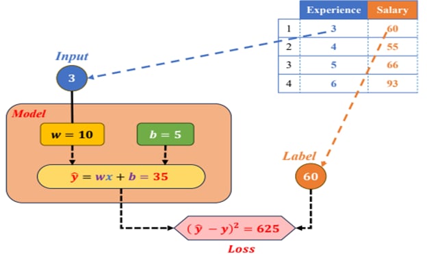
that represents the relationship between Experience (years) and Salary (in thousands).
| Index | Experience (x) | Salary (y) |
|---|---|---|
| 1 | 3 | 60 |
| 2 | 4 | 55 |
| 3 | 5 | 66 |
| 4 | 6 | 93 |
Table: Training data for Linear Regression.
Step 1: Initialize the Model
We start by initializing the model parameters:
$$
w = 10, \quad b = 5
$$
The hypothesis (prediction function) of Linear Regression is given by:
$$
\hat{y} = wx + b
$$
Substituting the initial parameters, we get:
$$
\hat{y} = 10x + 5
$$
Step 2: Compute the Prediction and Loss for One Sample
For the first sample (Index = 1), the experience value is $x = 3$ and the actual salary is $y = 60$.
$$ \hat{y} = 10(3) + 5 = 35 $$
The predicted salary is therefore $\hat{y} = 35$.
To measure the error, we calculate the loss using the Mean Squared Error (MSE) formula for a single sample:
$$ L(\hat{y}, y) = (\hat{y} - y)^2 $$
Substituting the values:
$$
L = (35 - 60)^2 = 625
$$
Step 3: Compute the Loss for All Samples
Repeating the same process for all four data points:
| Experience (x) | Salary (y) | Predicted $\hat{y}$ | Error $(\hat{y} - y)$ | Loss $(\hat{y} - y)^2$ |
|---|---|---|---|---|
| 3 | 60 | 35 | -25 | 625 |
| 4 | 55 | 45 | -10 | 100 |
| 5 | 66 | 55 | -11 | 121 |
| 6 | 93 | 65 | -28 | 784 |
Table: Computation of predicted values and losses for each data point.
The total loss over all samples is:
$$
L_{\text{total}} = 625 + 100 + 121 + 784 = 1630
$$
Step 4: Compute the Derivatives
Next, we compute the gradients (partial derivatives) of the loss function with respect to the parameters $w$ and $b$.
$$ \frac{\partial L}{\partial w} = \frac{\partial (\hat{y} - y)^2}{\partial w} = \frac{\partial (\hat{y} - y)^2}{\partial \hat{y}} \cdot \frac{\partial \hat{y}}{\partial w} $$
Since $\hat{y} = wx + b$, we have:
$$
\frac{\partial \hat{y}}{\partial w} = x
$$
Therefore:
$$
\frac{\partial L}{\partial w} = 2(\hat{y} - y)x
$$
Similarly, the derivative with respect to $b$ is:
$$
\frac{\partial L}{\partial b} = 2(\hat{y} - y)
$$
Step 5: Update the Parameters
Using the computed gradients, we update the model parameters as follows:
$$
w_{\text{new}} = w_{\text{old}} - \eta \frac{\partial L}{\partial w},
\qquad
b_{\text{new}} = b_{\text{old}} - \eta \frac{\partial L}{\partial b}
$$
where $\eta$ (eta) is the learning rate, controlling how large the update step is in each iteration.
Step 6: Interpretation
After substituting the calculated gradients and applying one update step,
we obtain new values of $w_{\text{new}}$ and $b_{\text{new}}$.
This process continues iteratively across multiple epochs until the loss converges to a minimal value.
Through this example, we can observe that:
- The initial loss ($L_{\text{total}} = 1630$) is quite high.
- After updating the parameters, the loss gradually decreases over time.
- The model converges after several iterations, achieving a better fit between predicted and actual values.
Chưa có bình luận nào. Hãy là người đầu tiên!