From Raw Data to Models: A Comprehensive Guide to Data Preprocessing

I. Introduction to Data Cleaning and Preprocessing

1. The Importance of Data Cleaning and Preprocessing

Figure 1. Data Cleaning

• Data cleaning and preprocessing are two essential and time-consuming stages in any data science workflow. This is because real-world data is often messy and incomplete. According to the principle of garbage in, garbage out, feeding poor-quality data into predictive models will inevitably reduce their accuracy.

• Therefore, by transforming raw data into a structured and more usable format, we can perform more accurate analysis. The quality of the input data directly determines the quality of the output results. Investing significant time in data preparation helps avoid misleading conclusions and prevents the development of inefficient models.

2. Data Cleaning and Preprocessing Workflow

• A typical data cleaning and preprocessing workflow includes the following steps:

1. Data Collection: Gather raw data from multiple sources such as databases, APIs, web scraping, or manual input.

2. Data Cleaning: Process the collected data by detecting and correcting errors, removing duplicate or irrelevant records, and handling missing values.

3. Data Integration: Combine data from different sources into a unified structure and resolve any inconsistencies.

4. Data Transformation: Convert data into a suitable format for analysis. This includes encoding categorical variables, normalizing numerical features, and creating new features.

5. Data Reduction: Reduce the dimensionality of the data if necessary. This involves feature extraction and feature selection to focus only on the most important variables.

• This process is iterative, and you will often revisit these steps multiple times throughout your data science workflow.

3. Popular Python Libraries for Data Cleaning and Preprocessing

• Python is widely favored by data scientists due to its ease of use and rich ecosystem of supporting libraries. Two core libraries for data cleaning are Pandas and Numpy.

• In addition, other essential libraries that support this process include Matplotlib and Seaborn for data visualization, Scikit-learn for preprocessing and machine learning, and Missingno for handling missing data.

1. Pandas: provides powerful data structures and tools for working with data. It allows users to easily filter, sort, aggregate, and clean datasets.

# import pandas library
import pandas as pd

# read CSV file as DataFrame in pandas
df = pd.read_csv('Ten_file_cua_ban.csv')

# display first rows
df.head()

2. Numpy: offers tools for numerical computation, including high-performance arrays and advanced operations for efficient data manipulation.

# import numpy library
import numpy as np

# Create arrays in NumPy
arr = np.array([1, 2, 3, 4, 5])

# Perform element-wise operations
arr2 = arr * 2

3. Matplotlib: a visualization library capable of creating various types of plots such as line charts and bar charts. It serves as the foundation for data visualization, commonly used in EDA (Exploratory Data Analysis).

# import Matplotlib library
import matplotlib.pyplot as plt

# Create a simple line plot
plt.plot([1, 2, 3, 4, 5])
plt.title("Simple Line Plot")
plt.xlabel("x-axis")
plt.ylabel("y-axis")
plt.show()

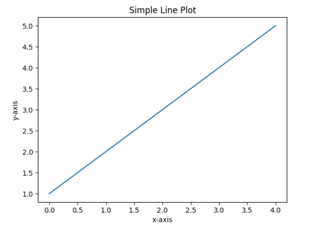
Figure 2. Simple line plot with Matplotlib Library

4. Seaborn: a data visualization library built on top of Matplotlib. It provides a higher-level interface that makes it easier to create visually appealing and informative statistical graphics.

# import Seaborn library
import seaborn as sns

# Load a sample dataset from the Seaborn library
df = sns.load_dataset('tips')

# Create a distribution plot
sns.histplot(df['total_bill'])
plt.title("Histogram of Total Bill")
plt.show()

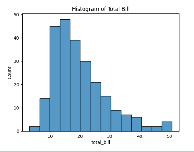
Figure 3. Histogram plot
5. Scikit-learn: provides a wide range of supervised and unsupervised learning algorithms. It also includes essential tools for model training, data preprocessing, feature selection, model evaluation, and many other useful utilities.

# Import the Scikit-learn library
from sklearn import datasets
from sklearn.model_selection import train_test_split
from sklearn.ensemble import RandomForestClassifier
from sklearn.metrics import accuracy_score

# Load the Iris dataset
iris = datasets.load_iris()

# Create feature and target arrays
X = iris.data
y = iris.target

# Split the data into training and testing sets
X_train, X_test, y_train, y_test = train_test_split(X, y, test_size=0.2, random_state=42)

# Initialize a Random Forest classifier (RandomForestClassifier) and train the model
clf = RandomForestClassifier(random_state=42)
clf.fit(X_train, y_train)

# Make predictions on the test dataset
y_pred = clf.predict(X_test)

# Evaluate the model accuracy
accuracy = accuracy_score(y_test, y_pred)
print("Accuracy:", accuracy)

6. Missingno: offers visualization tools for exploring the distribution of missing values. This is especially useful during data cleaning, helping you easily identify and handle missing information.

# Import missingno library
import missingno as msno
import pandas as pd
import numpy as np

# Create a sample DataFrame with missing values
df = pd.DataFrame({
    'Column1': [1, np.nan, 3, 4, 5],
    'Column2': [np.nan, np.nan, 7, 8, 9],
    'Column3': [10, 11, np.nan, np.nan, np.nan]
})

# Visualize missing values
msno.matrix(df)
plt.show()

Figure 4. Missingno matrix demo

• Each of these libraries provides a powerful set of tools that support different aspects of data cleaning, preprocessing, and data analysis.

II. Understanding Data Quality Issues

When entering the world of data science, one important reality we must accept is that we rarely encounter datasets that are perfectly cleaned and prepared. In most cases, raw datasets are filled with various data quality issues. This section explores how to identify common data quality problems, evaluate data quality and integrity, use (EDA) in the evaluation process, and handle duplicate and redundant data.

• Missing Data: This issue can arise from various causes such as human errors during data entry, failures in the data collection process, or situations where certain fields are not applicable. It is one of the most common data quality problems. Depending on the cause, missing values can lead to biased or inaccurate analysis. Therefore, handling missing data properly is crucial to maintaining model accuracy.

# Install required libraries
import pandas as pd

# Load your dataset
df = pd.read_csv('your_file_name.csv')

# Check for missing values in each column
missing_values = df.isnull().sum()
print(missing_values)

• Outliers: These are data points that differ significantly from the rest of the dataset. They may result from measurement errors, data entry mistakes, or they may be valid observations with extreme values. Outliers can greatly affect analysis results, so detecting and handling them is essential.

# Install required libraries
import seaborn as sns
import matplotlib.pyplot as plt

# Visualize outliers using a box plot
sns.boxplot(x=df['cot_cua_ban'])
plt.show()

A box plot visualizes the minimum value, quartiles, and maximum value of the data, helping to understand data distribution and identify outliers.

• Inconsistent Data Formats: This is a common issue caused by human errors, system changes, or merging data from multiple sources.

# Example: convert a column with numeric values stored as strings into numeric format
df['numeric_column'] = pd.to_numeric(df['numeric_column'], errors='coerce')

This command converts values in a numeric column into a proper numeric format. Non-numeric values are converted into NaN, helping maintain data integrity.

• Data Quality and Integrity Assessment: High-quality data is complete, accurate, and consistently formatted. In contrast, low-quality data contains errors, missing values, and inconsistencies. Data quality directly impacts analysis and predictive models, making it a critical step before any analysis or preprocessing.

• A simple yet powerful way to assess data quality is through (descriptive statistics). These metrics provide an overview of central tendency, variability, and data distribution.

# Use pandas to describe the dataset, providing an initial assessment of data quality
df.describe()

• Exploratory Data Analysis (EDA) for Data Quality Assessment: EDA is an approach used to analyze datasets in order to summarize their main characteristics, often using statistical charts and other data visualization techniques. This is a crucial step before proceeding to more advanced stages such as model building and prediction.

• One of the key aspects of EDA is visual exploration. Data visualization can provide new insights into your dataset. For example, a distribution plot can give a quick and overall view of how your data is distributed.

# Plot distribution histograms for all numerical columns in the dataset
df.hist(bins=50, figsize=(20, 15))
plt.show()

• Distribution plots can reveal important characteristics of the data. A bell-shaped and symmetric curve may indicate a normal distribution, while a skewed distribution may suggest the presence of outliers.

• Handling Duplicate and Redundant Data: These are two different issues that can appear in your dataset. Duplicate data refers to identical records, which can distort analysis results and lead to incorrect conclusions. Redundant data, on the other hand, does not add new information but can slow down computations and unnecessarily consume storage.

# Check for duplicate rows
duplicate_rows = df.duplicated()

# Count the number of duplicate rows
print(f"Number of duplicate rows: {duplicate_rows.sum()}")

# Remove duplicate values
df = df.drop_duplicates()

# Check the shape of the dataset after removal
print("Shape of DataFrame After Removing Duplicates:", df.shape)

• Handling duplicate and redundant data is an essential part of the data cleaning process and plays a critical role in maintaining the integrity of your analysis.

III. Handling Missing Data

Missing data is a common challenge that data scientists frequently encounter. Understanding how to identify and handle these gaps is extremely important because they can introduce bias or errors into your analysis. In this section, we will also explore several techniques for handling missing data.

1. Identifying and Understanding Missing Data

• Identifying missing data may sound simple - you just look for empty spaces. However, in real-world datasets, things are rarely that straightforward. Missing data can appear in many different forms, from obvious blank cells to placeholder values such as "N/A" or "-999", or even incorrectly entered values. Let’s discuss how to detect them using Python.

# Importing necessary library
import pandas as pd

# Checking for missing value
missing_value = df.isnull().sum()
print(missing_value)

• This code snippet prints the number of missing values in each column, giving you an initial overview of the extent and distribution of missingness in your dataset.

• Understanding missing data also requires knowing its categories. In statistics, missing data is generally divided into three types:

• Missing Completely at Random (MCAR): The missingness is not related to any other variable in the dataset. It occurs purely by chance.

• Missing at Random (MAR): The missingness of a variable is related to some other variables in the dataset, but not to the variable itself.

• Missing Not at Random (MNAR): The missingness of a variable is directly related to the value of that variable itself.

• The type of missing data will help guide your choice of the most appropriate handling technique.

2. Techniques for Handling Missing Data

• Deletion: This is the simplest method, which involves removing data entries that contain missing values altogether. However, this approach is only recommended when your data is MCAR and the proportion of missing values is very small compared to the overall dataset. Below is how you can do this using pandas:

# Drop columns with missing values
df.dropna(inplace=True)

• Data Imputation: This is the process of replacing missing data with substitute values. Common approaches include:

• Mean / Median / Mode Imputation: Replace missing values with the mean (for continuous data), median (for ordinal data), or mode/the most frequent value (for categorical data). However, this method may reduce the variance of the dataset and affect correlations with other variables.

# Impute missing values with the mean
df.fillna(df.mean(), inplace=True)

• Constant Value Imputation: Replace missing values with a fixed constant. This can be useful when you have enough domain knowledge to make a reasonable assumption about the missing values.

# Impute missing values with a fixed constant
df.fillna(0, inplace=True)

• Predictive Model Imputation: Use statistical models or machine learning algorithms to predict missing values based on other available data. Although this approach can provide higher accuracy, it is also more complex.

# Impute missing values using a predictive model with Linear Regression
from sklearn.linear_model import LinearRegression

# Split the data into two subsets: one with missing values and one without missing values
missing = df[df['A'].isnull()]
not_missing = df[df['A'].notnull()]

# Initialize the model
model = LinearRegression()

# Train the model (using other columns to learn patterns for predicting column 'A')
model.fit(not_missing.drop('A', axis=1), not_missing['A'])

# Predict the missing values
predicted = model.predict(missing.drop('A', axis=1))

# Fill the predicted values back into the missing positions in the original dataset
df.loc[df['A'].isnull(), 'A'] = predicted

3. Introduction to Pandas for Handling Missing Data

• As shown in the examples above, pandas is a powerful library for handling missing data. The methods isnull() and notnull() are very useful for identifying missing values. The fillna() method helps fill in missing data. You have already seen it used for constant and mean imputation, but it is much more flexible than that. For example, you can fill missing values using the previous valid value in the sequence (with method="ffill" - Forward Fill) or the next valid value (with method="bfill" - Backward Fill).

# Fill missing values using the next valid value
df.fillna(method='ffill', inplace=True)

# Fill missing values using the previous valid value
df.fillna(method='bfill', inplace=True)

• Advanced Techniques for Handling Missing Data: These can be applied when you need to consider relationships between features or when your dataset contains many missing values scattered across different records.

• Multivariate Imputation: This is a statistical technique for handling missing data, where missing values are estimated multiple times. The process generates multiple complete datasets, each of which is analyzed separately, and the results are then combined into a single final result. A commonly used method is MICE (Multivariate Imputation by Chained Equations), which accounts for the uncertainty surrounding missing values.

# Perform multivariate imputation using chained equations
from sklearn.experimental import enable_iterative_imputer
from sklearn.impute import IterativeImputer

# Initialize the MICE imputer
mice_imputer = IterativeImputer()

# Apply the imputation process
df_imputed = mice_imputer.fit_transform(df)

• Predictive Model Imputation: This approach uses machine learning models to predict missing values. While a linear regression model may be sufficient in some cases, more advanced methods such as decision trees, random forests, or neural networks may perform better depending on the complexity of your data.

# Impute missing values using a Random Forest model
from sklearn.ensemble import RandomForestRegressor

# Prepare the data: split into subsets with and without missing values
missing = df[df['A'].isnull()]
not_missing = df[df['A'].notnull()]

# Initialize the model (set 100 decision trees for prediction)
model = RandomForestRegressor(n_estimators=100, random_state=0)

# Train the model (learn patterns from available data)
model.fit(not_missing.drop('A', axis=1), not_missing['A'])

# Predict missing values
predicted = model.predict(missing.drop('A', axis=1))

# Fill the predicted values into the missing positions in the original DataFrame
df.loc[df['A'].isnull(), 'A'] = predicted

IV. Dealing with Outliers

1. Outliers

Outliers are unusual observations that have values significantly different (either much smaller or much larger) from the rest of the dataset. They may arise due to natural variation or errors in measurement/data entry. While outliers can sometimes indicate important discoveries or issues in the data collection process, they can also distort the data and lead to misleading results.

Understanding outliers is crucial because their presence can have significant impacts on data analysis. They can:

• Affect the Mean and Standard Deviation: Outliers can significantly shift the mean and inflate the standard deviation, distorting the overall distribution of the data.

• Impact Model Accuracy: Many machine learning algorithms are sensitive to the scale and distribution of feature values. Outliers can distort the training process, leading to longer training times and less accurate models.

2. Techniques for Detecting Outliers

Outliers can be detected using several methods, each with its own advantages and limitations. Below are some commonly used approaches:

• Statistical Methods

• Z-score: The Z-score measures how many standard deviations a data point is away from the mean.

In an ideal normal distribution:

• The range [-1, 1] contains approximately 68% of the data.
• The range [-2, 2] contains approximately 95% of the data.
• The range [-3, 3] contains approximately 99.7% of the data.

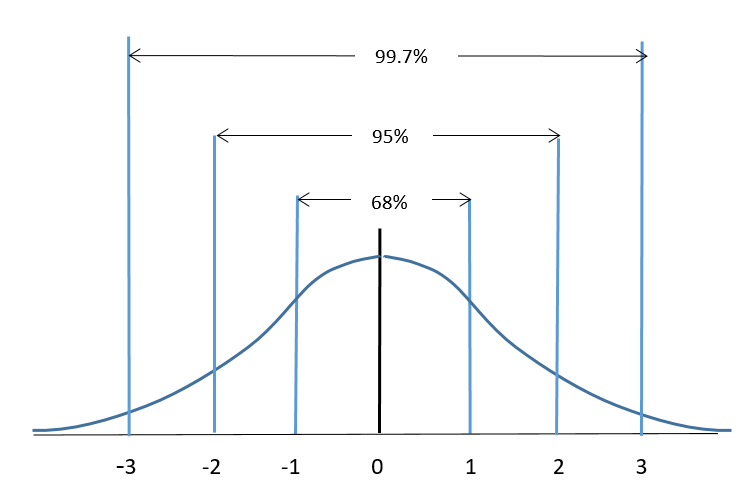
Figure 5. Ideal normal distribution

Note: A common rule of thumb is that a data point with a Z-score greater than 3 or less than -3 is considered an outlier.

• Interquartile Range (IQR) Method: This method identifies outliers as data points that fall below the first quartile (Q1) or above the third quartile (Q3) by a certain multiple of the IQR.

• A box plot describes key characteristics of a dataset such as central tendency, dispersion, and symmetry, and is also an effective way to detect outliers. It displays the quartiles Q1, Q2 (median), Q3, along with the minimum and maximum values.

• One edge of the box corresponds to Q1, while the opposite edge corresponds to Q3. The interquartile range is defined as IQR = Q3 - Q1.

• From Q1, a line extends toward the lower bound of the data with a length of 1.5 × IQR, and from Q3, another line extends toward the upper bound with the same length (these are called the “lower whisker” and “upper whisker”). Data points outside the box and whiskers are typically marked as individual points (“o”) and are considered outliers.

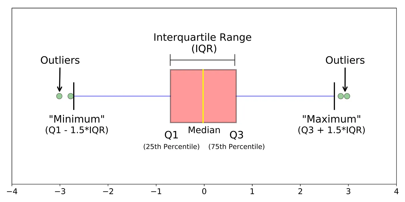
Figure 6. Interquartile Range (IQR) Method
- Visualization

Box plots and scatter plots are excellent tools for visualizing and detecting outliers.

• Box plot: Refer to the section above

• Scatter plot:

Concept: Data is displayed as a collection of points. Each point represents two variables - one determines the position on the horizontal axis (X-axis), and the other determines the position on the vertical axis (Y-axis).

Note: In a scatter plot, outliers are clearly visible. They appear as points that are isolated and far away from the general cluster or trend of the data.

import matplotlib.pyplot as plt

# Sample data
x = [5,7,8,7,2,17,2,9,4,11,12,9,6]   # car age
y = [99,86,87,88,111,150,138,87,94,78,77,85,86]   # speed of each car

# Create a figure with 1 row and 2 columns
plt.figure(figsize=(12, 5))

# 1. Plot Scatter Plot
plt.subplot(1, 2, 1)
plt.scatter(x, y)
plt.title("Scatter Plot")
plt.xlabel("tuổi xe")
plt.ylabel("tốc độ")

# 2. Plot Box Plot for the variable Speed (y)
plt.subplot(1, 2, 2)
plt.boxplot(y)
plt.title("Box Plot")
plt.ylabel("tốc độ")

# Note: The box plot clearly shows that the value 150 is an outlier

# Display the plots
plt.tight_layout()
plt.show()

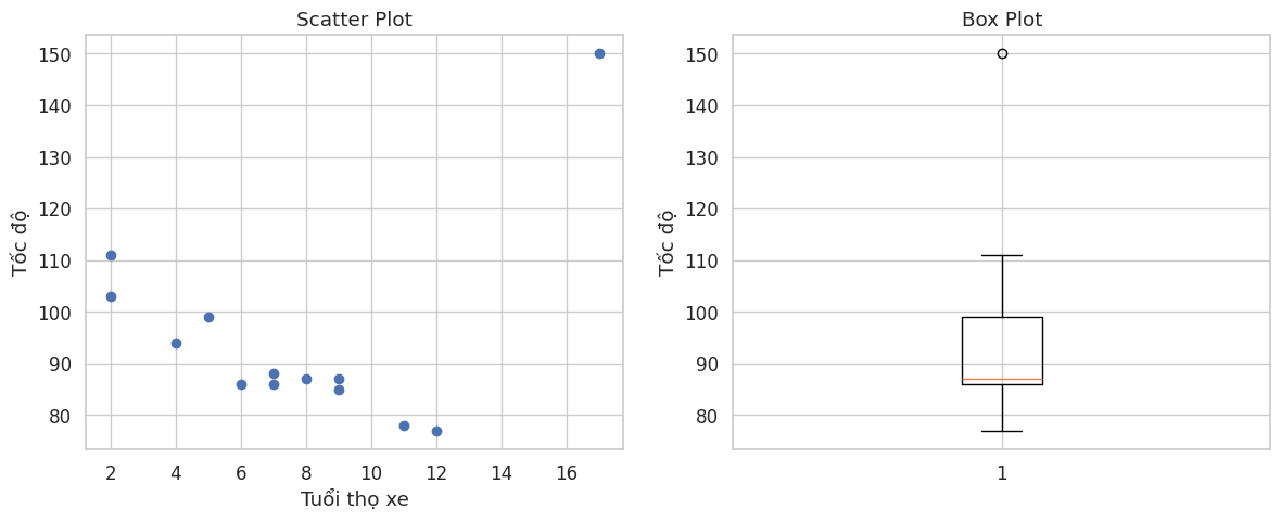
Figure 7. IQR method visualization

3. Strategies for Handling Outliers

There are several ways to handle outliers, and the appropriate method depends on the nature of the data and the specific problem you are solving. Below are some common strategies:

• Removal

Removing outliers is the simplest approach, but it should be used with caution. You should only remove an outlier if you are certain that it is caused by a data entry error or incorrect measurement. In some cases, removing valuable data points may lead to information loss and biased results.

# Filter out outliers
filtered_data = outlier_data[(z_scores <= 3)]

• Transformation

Transforming variables can help reduce the impact of outliers. Common transformations include logarithmic (log), square root, and inverse transformations. These methods compress larger values, thereby reducing the influence of extreme values.

# Apply inverse transformation
transformed_data = 1 / data

• Winsorization

In a Winsorized dataset, extreme values are replaced with specific percentiles (commonly the 5th and 95th percentiles). This technique preserves the dataset size, unlike removal.

from scipy.stats.mstats import winsorize

# Apply winsorization
winsorized_data = winsorize(outlier_data, limits=[0.05, 0.05])

• Machine Learning Models

Some machine learning models, such as Random Forests and Support Vector Machines (SVM), are less sensitive to outliers. Using these models can be a practical strategy when working with data that contains outliers.

V. Data Normalization and Scaling

In data preprocessing, an essential step is normalization and scaling. These techniques help standardize the range of independent variables or features in a dataset.

1. Understanding the Importance of Data Normalization and Scaling

Machine learning algorithms perform better when input variables are on a similar scale. Without normalization or scaling, features with larger values can dominate the model’s results. This may lead to biased outcomes and prevent the model from properly capturing the influence of other features.

Normalization and scaling bring different features to the same scale, allowing for fair comparison and ensuring that no single feature dominates the others. Moreover, these techniques can speed up the training process. For example, gradient descent converges faster when features are on similar scales.

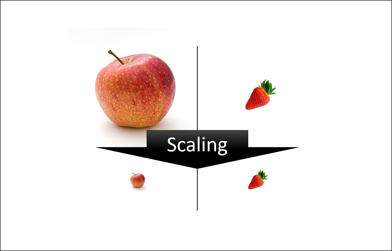
Figure 8. Scaling method example
For instance, a feature like age is typically on a very different scale compared to salary. Since salary values are usually much larger, any combined calculations may be dominated by the salary feature.

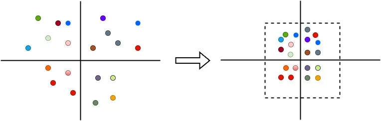
Figure 9. Data Normalization example

2. Data Normalization Techniques

Data normalization is a method used to transform numerical features in a dataset to a common scale. Below are some common normalization techniques:

• Min-max scaling:

Min-max scaling is one of the simplest normalization methods. It rescales and shifts each feature individually so that its values fall within the range [0, 1].

Formula:
- Min-max scaling:

$$ x' = \frac{x - x_{min}}{x_{max} - x_{min}} $$

where:
- $x$: original value
- $x_{min}$: minimum value of the feature
- $x_{max}$: maximum value of the feature

Example code:

from sklearn.preprocessing import MinMaxScaler

# Example with a simple dataset
data = np.array([1, 2, 3, 4, 5, 6, 7, 8, 9, 10]).reshape(-1, 1)
scaler = MinMaxScaler()
normalized_data = scaler.fit_transform(data)

3. Z-score Normalization

This technique standardizes features so that they have a mean of 0 and a standard deviation of 1. It transforms the data distribution to be centered around 0 with unit variance.
Formula:
- Z-score normalization (Standardization):

$$ x' = \frac{x - \mu}{\sigma} $$

where:
- $\mu$: mean
- $\sigma$: standard deviation
Example code:

from sklearn.preprocessing import StandardScaler

# Example with a simple dataset
data = np.array([1, 2, 3, 4, 5, 6, 7, 8, 9, 10]).reshape(-1, 1)
scaler = StandardScaler()
standardized_data = scaler.fit_transform(data)

4. Feature Scaling Techniques

Feature scaling is a general term for methods that adjust the range of a feature. In addition to the normalization techniques mentioned above, the following method is also commonly used:

• Robust scaling

Robust scaling is similar to min-max scaling but uses the interquartile range (IQR) instead of the minimum and maximum values, making it less sensitive to outliers.

Formula:
- Robust Scaling (based on IQR):

$$ x' = \frac{x - Q_1}{Q_3 - Q_1} $$

or commonly written as:

$$ x' = \frac{x - \text{median}}{IQR} $$

where:
- $Q_1$: first quartile
- $Q_3$: third quartile
- $IQR = Q_3 - Q_1$
- median ($Q_2$): median value

Example code:

from sklearn.preprocessing import RobustScaler

# Example with a simple dataset
data = np.array([1, 2, 3, 4, 5, 6, 7, 8, 9, 10]).reshape(-1, 1)
scaler = RobustScaler()
robust_scaled_data = scaler.fit_transform(data)

VI. Feature Selection and Extraction

Feature selection and feature extraction are critical steps in the data preprocessing pipeline for machine learning and data science projects. These techniques can make the difference between a highly effective model and a completely failed one.

They are used to reduce the dimensionality of data, thereby improving computational efficiency and potentially enhancing model performance.

1. Feature Selection

Feature selection is the process of selecting a subset of the most important features and removing the rest for model building. This is important for several reasons:

• Simplicity: Fewer features make the model simpler and easier to interpret.
• Speed: Less data means faster training for algorithms.
• Preventing overfitting: Reducing redundant features lowers the chance of learning noise instead of meaningful patterns.

2. Feature Extraction

On the other hand, feature extraction is the process of transforming or mapping high-dimensional data into a lower-dimensional space. Unlike feature selection, which retains original features, feature extraction creates new features that represent most of the useful information from the original data. The benefits include:

• Dimensionality reduction: Fewer features help speed up training.
• Better performance: In some cases, models perform better in the transformed feature space.

3. Feature Selection Techniques

Feature selection methods are generally divided into three categories: filter methods, wrapper methods, and embedded methods.

• Filter Methods

These methods evaluate each feature based on its statistical relationship with the target variable (output/label), then retain the highest-scoring features. Common scoring techniques include chi-squared test, information gain, and correlation coefficient.

Step-by-step process:

1. Take all features from the original dataset
2. Compute a score for each feature using a statistical test to measure its relationship with the target variable (y)
3. Rank the features based on their scores and select the top-k features
4. Feed the selected features into the machine learning model

• Wrapper Methods

Unlike filter methods, wrapper methods use machine learning models to evaluate the quality of different feature subsets. They treat feature selection as a search problem - testing multiple combinations of features, training a model for each combination, evaluating performance, and selecting the best subset. Two common techniques are Forward Selection và Recursive Feature Elimination (RFE).

• Embedded Methods

Embedded methods integrate feature selection directly into the model training process. Unlike filter (pre-training selection) and wrapper (external selection), embedded methods perform selection during training.

The main mechanism is regularization, which adds a penalty term to the model’s objective function, forcing less important feature coefficients toward zero (or exactly zero). Two common regularization techniques are Lasso and Ridge.

4. Feature Extraction Techniques

Unlike the methods above, feature extraction creates new features by combining and transforming the original ones. The result is a compressed feature space (lower dimensionality) that still preserves most of the useful information. Common dimensionality reduction techniques include PCA and t-SNE.

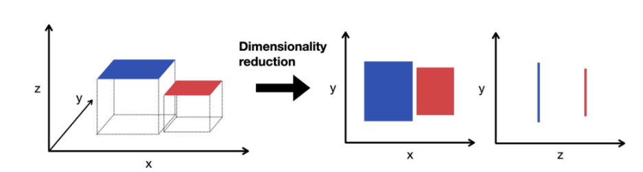
Figure 10. Dimensionality reduction example

• PCA (Principal Component Analysis): Identifies new axes (called principal components) that capture the maximum variance in the data, then projects the data onto these axes. For example, three original features can be reduced to two new features (PC1, PC2) while preserving most of the information.

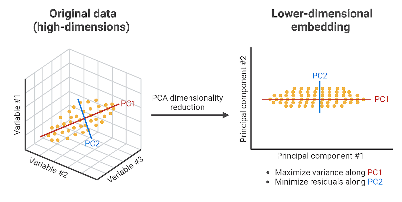
Figure 11. Principal dimensionality reduction

• t-SNE: Works differently by preserving the “neighborhood” relationships between data points when projecting them into a lower-dimensional space. Points that are close in the original space remain close after transformation, resulting in clearly visible clusters.

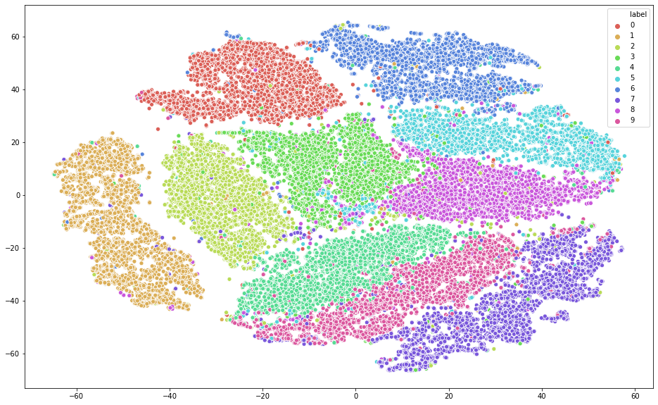
Figure 12. t-SNE method
Note: t-SNE is mainly used for visualization, not for model training, because its results vary between runs and it cannot be directly applied to new data.

VII. Encoding Categorical Variables

Categorical variables are a common type of non-numeric data and play an important role in many data science and machine learning applications. Encoding categorical data is a crucial step in the data preprocessing stage. In this section, we will explore what categorical variables are, the challenges they present, different encoding techniques, and how to handle high cardinality and rare categories.

1. Understanding Categorical Variables and Their Challenges

Categorical variables represent data that can be divided into groups. Examples include race, gender, age group, and education level. Although the last two can be continuous variables, they are often treated as categorical in practice.

Categorical variables pose challenges when building machine learning models because these models are inherently mathematical and require numerical input. Therefore, categorical variables must be converted into a suitable numeric format—a process known as categorical encoding.

However, not all encoding methods are suitable for every problem. The choice of technique depends on the characteristics of the data and the type of model being used. Additionally, some encoding methods can significantly increase the dimensionality of the dataset, leading to longer training times and a higher risk of overfitting.

2. Categorical Encoding Techniques

There are many ways to encode categorical variables, each with its own advantages and disadvantages. Here, we focus on two commonly used techniques: one-hot encoding and label encoding.

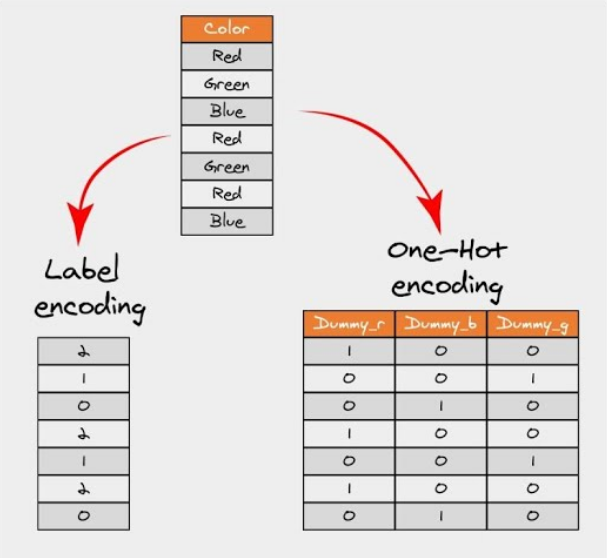
Figure 13. Categorical Encoding Example

• One-hot encoding: This method transforms categorical variables into a format that machine learning algorithms can use effectively. Each category is converted into a new column and assigned a binary value (1 or 0). Each value is represented as a binary vector.

import pandas as pd

data = {
    'name': ['John', 'Lisa', 'Peter', 'Carla', 'Eva', 'John'],
    'sex': ['male', 'female', 'male', 'female', 'female', 'male'],
    'city': ['London', 'London', 'Paris', 'Berlin', 'Paris', 'Berlin']
}

df = pd.DataFrame(data)

df_one_hot = pd.get_dummies(df, columns=['sex'], prefix='sex')

print("Original DataFrame:")
print(df)

print("\nDataFrame after one-hot encoding 'sex' and label encoding 'city':")
print(df_one_hot)

• Label encoding: Label encoding is a popular technique where each category is assigned a unique integer based on alphabetical order.

import pandas as pd
from sklearn.preprocessing import LabelEncoder

data = {
    'name': ['John', 'Lisa', 'Peter', 'Carla', 'Eva', 'John'],
    'sex': ['male', 'female', 'male', 'female', 'female', 'male'],
    'city': ['London', 'London', 'Paris', 'Berlin', 'Paris', 'Berlin']
}

df = pd.DataFrame(data)

le = LabelEncoder()
df['city_encoded'] = le.fit_transform(df['city'])

print(df)

3. Handling High Cardinality and Rare Categories

High cardinality refers to categorical features with a large number of unique values, which can create challenges for certain encoding methods. For example, applying one-hot encoding to such features can dramatically increase the number of columns, leading to higher memory usage.

One way to handle high cardinality is to group infrequent values into a common category called “Other.” This approach also helps address the issue of rare categories - values that appear in the training data but are unlikely to appear in real-world data later.

import pandas as pd
from sklearn.preprocessing import LabelEncoder

data = {
    'name': ['John', 'Lisa', 'Peter', 'Carla', 'Eva', 'John'],
    'sex': ['male', 'female', 'male', 'female', 'female', 'male'],
    'city': ['London', 'London', 'Paris', 'Berlin', 'Paris', 'Berlin']
}

df = pd.DataFrame(data)

# Handle high cardinality and rare categories in 'name' column
counts = df['name'].value_counts()
other = counts[counts < 2].index  # here we consider names appearing less than 2 times as "rare"

df['name'] = df['name'].replace(other, 'Other')

print("\nDataFrame after handling high cardinality and rare categories in 'name' column:")
print(df)

Example Python Code for Categorical Encoding

Below is a complete example of how to encode a categorical feature in a dataset:

import pandas as pd
from sklearn.preprocessing import LabelEncoder

# Let's create a simple DataFrame
data = {
    'name': ['John', 'Lisa', 'Peter', 'Carla', 'Eva', 'John'],
    'sex': ['male', 'female', 'male', 'female', 'female', 'male'],
    'city': ['London', 'London', 'Paris', 'Berlin', 'Paris', 'Berlin']
}

df = pd.DataFrame(data)

# One-hot encode the 'sex' column
df_one_hot = pd.get_dummies(df, columns=['sex'], prefix='sex')

# Label encode the 'city' column
le = LabelEncoder()
df['city_encoded'] = le.fit_transform(df['city'])

# Display the original DataFrame and the modified DataFrame
print("Original DataFrame:")
print(df)

print("\nDataFrame after one-hot encoding 'sex' and label encoding 'city':")
print(df_one_hot)

# Handle high cardinality and rare categories in 'name' column
counts = df['name'].value_counts()
other = counts[counts < 2].index  # here we consider names appearing less than 2 times as "rare"

df['name'] = df['name'].replace(other, 'Other')

print("\nDataFrame after handling high cardinality and rare categories in 'name' column:")
print(df)

In this example, we start with a simple DataFrame containing the columns: name, sex, and city. We then apply one-hot encoding to the sex column using the get_dummies function from pandas, and label encoding to the city column using LabelEncoder from the scikit-learn library. The result is a DataFrame where both sex and city have been converted into numerical formats suitable for machine learning models.

Next, we handle high cardinality and rare categories in the name column. We count the frequency of each name using the value_counts function and identify names that appear fewer than two times as “rare.” These rare names are then replaced with the label “Other.”

The output of the code demonstrates how categorical variables can be effectively transformed for modeling.

Categorical encoding is a crucial step in data preprocessing, and selecting the appropriate method based on your data and model can significantly impact model performance.

VIII. Handling Imbalanced Data

Imbalanced data is a common issue in machine learning, where the number of observations in one class is significantly lower than in others. In this section, we will explore what imbalanced data is, its impact on machine learning models, and various techniques to handle it.

1. Understanding Imbalanced Data and Its Impact on Machine Learning

Imbalanced data, as the name suggests, occurs in classification problems where class distributions are not equal. For example, in a binary classification problem, you may have 100 samples, where 90 belong to class ‘A’ (majority class) and only 10 belong to class ‘B’ (minority class). This is a typical example of imbalanced data.

The main issue with imbalanced data is that most machine learning algorithms perform best when class distributions are relatively balanced. Since these algorithms are often designed to maximize accuracy and minimize error, they tend to focus on the majority class and ignore the minority class. As a result, a model may predict only the majority class and still achieve high accuracy, which is not useful because the minority class - often the class of interest - is completely overlooked.

2. Techniques for Handling Imbalanced Data

There are several strategies to handle imbalanced data, which can be grouped into three main categories: resampling techniques, cost-sensitive learning, and ensemble methods.

• Resampling Techniques: Resampling is the simplest way to handle imbalanced data. It includes removing samples from the majority class (undersampling) and/or increasing samples in the minority class (oversampling).

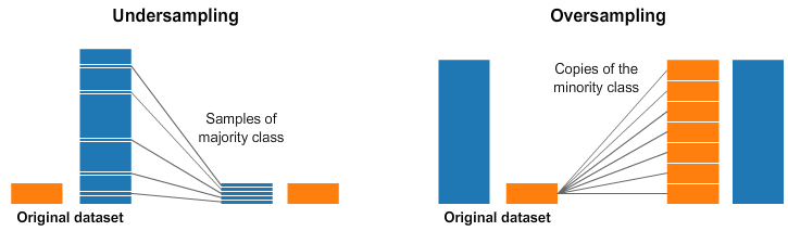
Figure 14. Resampling Techniques example

from imblearn.over_sampling import RandomOverSampler
from imblearn.under_sampling import RandomUnderSampler

# Assuming 'X' is your feature set and 'y' is the target variable
ros = RandomOverSampler()
X_resampled, y_resampled = ros.fit_resample(X, y)

rus = RandomUnderSampler()
X_resampled, y_resampled = rus.fit_resample(X, y)

• Cost-Sensitive Learning: This approach incorporates misclassification costs (false positives and false negatives) into the learning algorithm. In other words, it assigns a higher penalty to misclassifying the minority class, encouraging the model to pay more attention to it.

from sklearn.svm import SVC

# Create a SVC model with 'balanced' class weight
clf = SVC(class_weight='balanced')
clf.fit(X, y)

• Ensemble Methods: Ensemble methods, such as Random Forest and boosting algorithms, can also be used to handle imbalanced data. These methods work by combining multiple models to produce a final prediction.

from sklearn.ensemble import RandomForestClassifier

# Create a random forest classifier
clf = RandomForestClassifier()
clf.fit(X, y)

Example Python Code for Handling Imbalanced Data

We can use Python and various libraries to handle imbalanced datasets.

import pandas as pd
from sklearn.model_selection import train_test_split
from sklearn.metrics import classification_report
from sklearn.ensemble import RandomForestClassifier
from imblearn.over_sampling import SMOTE

data = pd.read_csv("train.csv")

X = data.drop("Churn", axis=1)
y = data["Churn"]

# One-hot encode categorical columns
X = pd.get_dummies(X, drop_first=True)

x_train, x_test, y_train, y_test = train_test_split(
    X, y, test_size=0.2, random_state=42, stratify=y
)

print("Before SMOTE:")
print(y_train.value_counts())

sm = SMOTE(random_state=42)
X_train_res, y_train_res = sm.fit_resample(x_train, y_train)

print("\nAfter SMOTE:")
print(y_train_res.value_counts())

clf = RandomForestClassifier(random_state=42, n_estimators=200)
clf.fit(X_train_res, y_train_res)

y_pred = clf.predict(x_test)

print("\nClassification Report:")
print(classification_report(y_test, y_pred))

In this example, we use a popular oversampling technique called SMOTE (Synthetic Minority Over-sampling Technique). SMOTE works by selecting samples that are close to each other in the feature space, drawing a line between them, and generating new samples along that line.

Figure 15. SMOTE method

Specifically, a random sample from the minority class is selected first. Then, its k nearest neighbors (typically k = 5) are identified. A random neighbor is chosen, and a new sample is created at a random point along the line connecting the two points in the feature space.

This method is effective because the generated samples are realistic - they lie close to existing minority class samples in the feature space.

In the final part of the code, we build a Random Forest classifier, train it on the resampled dataset, make predictions on the test set, and print a classification report to evaluate the results.

This section provides an overview of the challenges and strategies for handling imbalanced data. While it covers commonly used methods, it is important to note that the optimal technique depends on the specific characteristics of the dataset and the problem. Understanding these methods is essential for effectively handling imbalanced datasets and building robust and reliable machine learning models.

IX. Data Integration and Transformation Techniques

In practice, data is often scattered across multiple sources, each with its own structure and format. Even when data is centralized, it may not be in an optimal format for analysis or modeling. This section discusses data integration and transformation techniques that help make data more suitable for analysis.

1. Data Integration Methods

Data integration is the process of combining data from multiple sources to provide a unified view. This process is important in many scenarios, including business applications (e.g., merging databases from two companies) and scientific research (e.g., combining results from different biological data repositories).

• Merging: Merging combines two or more datasets based on common columns.

# Assuming 'df1' and 'df2' are your dataframes
merged_df = pd.merge(df1, df2, on='common_column')

• Joining: Joining is a convenient way to combine columns from two DataFrames that may have different indices into a single resulting DataFrame. In pandas, this can be done using the join function.

# Assuming 'df1' and 'df2' are your dataframes
joined_df = df1.join(df2, lsuffix='_df1', rsuffix='_df2')

• Concatenating: Concatenation is the process of combining datasets by adding DataFrames along a particular axis, either row-wise or column-wise.

# Assuming 'df1' and 'df2' are your dataframes
concat_df = pd.concat([df1, df2])

2. Data Transformation Techniques

Data transformation is the process of converting data from one format or structure into another.

• Binning: Binning is a transformation technique used to group continuous values into intervals (bins) or buckets. This is especially useful for handling noise or outliers.

# Assuming 'df' is your dataframe and 'age' is the column to bin
bins = [0, 18, 35, 60, np.inf]
names = ['<18', '18-35', '35-60', '60+']

df['age_range'] = pd.cut(df['age'], bins, labels=names)

• Log Transformation: Log transformation replaces each variable $x$ with $log(x)$. The choice of the logarithm base is typically determined by the analyst and depends on the purpose of the statistical model.

# Assuming 'df' is your dataframe and 'price' is the column to transform
df['log_price'] = np.log(df['price'])

• Power Transformation: Power transformation is a statistical technique used to make data more closely follow a normal distribution.

from sklearn.preprocessing import PowerTransformer

# Assuming 'X' is your feature set
pt = PowerTransformer()
X_transformed = pt.fit_transform(X)

3. Handling Skewed Distributions and Nonlinear Relationships

In statistics, skewness measures the asymmetry of a probability distribution relative to its mean. It indicates both the direction and degree of deviation from symmetry, and can be positive, negative, or undefined.

To handle skewed data, transformations such as logarithmic, square root, or cube root are commonly applied to normalize the distribution.

# Log transformation to handle right skewness
# Assuming 'df' is your dataframe and 'income' is the skewed feature
df['log_income'] = np.log(df['income'] + 1)  # We add 1 to handle zero incomes

# Confirming the change in skewness
print("Old skewness:", df['income'].skew())
print("New skewness:", df['log_income'].skew())

Nonlinear relationships between variables can be addressed in several ways. One common approach is to use polynomial features, where features are raised to higher powers to capture more complex relationships.

from sklearn.preprocessing import PolynomialFeatures

# Assuming 'X' is your feature set
poly = PolynomialFeatures(degree=2)
X_poly = poly.fit_transform(X)

This section provides an overview of data integration and transformation techniques - essential components of data preprocessing. Understanding these techniques is crucial, as real-world data often requires multiple steps of cleaning, preprocessing, and transformation to uncover meaningful patterns and insights.

Conclusion

The content presented above provides a systematic overview of the key steps in the data cleaning and preprocessing pipeline - a foundational stage that is often underestimated in data science. From identifying data quality issues such as missing values, duplicate data, and outliers, to applying advanced techniques like normalization, categorical encoding, dimensionality reduction, and handling imbalanced data, each step plays a critical role in determining the final performance of a model.

One important point to emphasize is that there is no “one-size-fits-all” solution for every problem. The choice of appropriate preprocessing techniques depends heavily on the nature of the data, the analysis objectives, and the type of model being used. For example, handling missing data requires balancing accuracy and complexity; dealing with outliers requires distinguishing between noise and valuable information; and selecting an encoding method can directly impact dimensionality and the risk of overfitting.

In addition, techniques such as feature selection, feature extraction, and scaling not only improve model performance but also help reduce computational costs and enhance interpretability. In practice, data preprocessing is often an iterative process - you may need to revisit and refine multiple steps before achieving optimal results.

Ultimately, it can be concluded that: the quality of input data directly determines the quality of the output model. A well-designed preprocessing pipeline not only improves model performance but also deepens your understanding of the data - a core element in any data science problem.

REFERENCES

Géron, A. (2019). Hands-on machine learning with scikit-learn, keras, and tensorflow (2nd ed.). O'Reilly Media. https://www.oreilly.com/library/view/hands-on-machine-learning/9781492032632/

McKinney, W. (2022). Python for data analysis (3rd ed.). O'Reilly Media. https://wesmckinney.com/book/

Pedregosa, F., Varoquaux, G., Gramfort, A., Michel, V., Thirion, B., Grisel, O., ... Duchesnay, E. (2011). Scikit-learn: Machine learning in Python. Journal of Machine Learning Research, 12, 2825–2830. https://jmlr.org/papers/v12/pedregosa11a.html

The pandas development team. (2023). Pandas: powerful Python data analysis toolkit. Pandas documentation. https://pandas.pydata.org/docs/

Chawla, N. V., Bowyer, K. W., Hall, L. O., & Kegelmeyer, W. P. (2002). SMOTE: Synthetic minority over-sampling technique. Journal of Artificial Intelligence Research, 16, 321–357. https://doi.org/10.1613/jair.953

AI ML Analytics. (2024). Feature scaling [Image]. AI ML Analytics. https://ai-ml-analytics.com/feature-scaling

Babbar, T. (2023). Beyond the norm: How outlier detection transforms data analysis [Image]. AlliedOffsets. https://blog.alliedoffsets.com/beyond-the-norm-how-outlier-detection-transforms-data-analysis

Boutnaru, S. (2024). The artificial intelligence journey — PCA (principal component analysis) [Image]. Medium. https://medium.com/@boutnaru/the-artificial-intelligence-journey-pca-principal-component-analysis-80b4d12b2cd2

Mazur, I., & Moshenko, K. (2021). Business/technical mathematics illustration [Image]. BCcampus. https://pressbooks.bccampus.ca/businessmathematics/

Roy, B. (2020). All about feature scaling [Image]. Towards Data Science. https://towardsdatascience.com/all-about-feature-scaling-bcc0ad75cb35

Sampaio, F. (2023). Oversampling and undersampling techniques in fraud prevention [Image]. Medium. https://medium.com/@fernandasampaio_74014/oversampling-and-undersampling-techniques-in-fraud-prevention-53129148281a

Sharma, S. (2026). One hot encoding vs label encoding [Image]. GeeksforGeeks. https://www.geeksforgeeks.org/machine-learning/one-hot-encoding-vs-label-encoding/

Single-cell best practices developers. (2023). Dimensionality reduction [Image]. Single-cell best practices. https://www.sc-best-practices.org/preprocessing_visualization/dimensionality_reduction.html

Zhang, D. (2020). Dimensionality reduction using t-distributed stochastic neighbor embedding (t-SNE) on the MNIST dataset [Image]. Medium. https://medium.com/data-science/dimensionality-reduction-using-t-distributed-stochastic-neighbor-embedding-t-sne-on-the-mnist-9d36a3dd4521

Edure. (2024). Data cleaning illustration [Image]. Edure. https://edure.in/data-cleaning-in-data-science/