
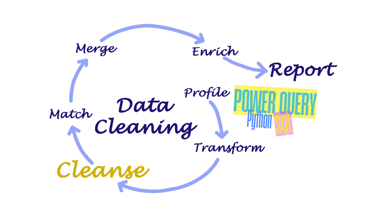
1. Retail Data Context and the GIGO Concept
1.1. Context
The modern retail industry is entering a digital era where data becomes a core asset that helps businesses make faster and more accurate decisions, while building sustainable competitive advantages. The growth of the omnichannel retail model drives continuous data generation from multiple sources such as Point of Sale (POS) systems, e-commerce platforms, loyalty programs, and inventory management systems. However, as data volume, velocity, and variety increase, the risk of errors, missing values, and inconsistencies rises as well.
In Vietnam, the shift toward omnichannel retail has accelerated. Many companies have started integrating data from physical stores and online channels to build a 360-degree customer profile, optimize inventory, and improve the shopping experience. Even so, channel data is often fragmented, making synchronization difficult and harming demand forecasting, operations planning, and long-term strategy.
In this context, data quality becomes a prerequisite. A modern analytics system cannot produce trustworthy results if the input data contains too many issues. That is why the concept of GIGO matters in practice.
1.2. The GIGO Concept
GIGO is short for Garbage In, Garbage Out - if the input is "garbage", the output will also be "garbage". This is a foundational principle in computer science and data analytics: output quality depends directly on input quality. No matter how advanced an algorithm is, if the input is wrong, incomplete, or noisy, the output can be meaningless or even lead to bad business decisions.
Historically, the idea appears early in the development of computing. Charles Babbage raised the point that a machine cannot produce a correct answer if the input is already incorrect. In 1957, William D. Mellin emphasized that computers cannot "think" to correct human errors. In the 1960s, IBM's George Fuechsel popularized the term GIGO to teach users the importance of accurate data entry.
In other words, GIGO is not just a technical slogan; it is a core principle of every modern analytics system. To produce reliable reports, strong models, and confident decisions, the first step is to clean the input data.
2. The Role of Data Cleaning
2.1. What Is Data Cleaning?
Data cleaning is the process of improving raw data quality by increasing accuracy, consistency, and usability. In real-world projects, data collected from multiple systems often contains missing values, duplicates, formatting issues, invalid records, and irrelevant noise. If these problems are not handled, they directly reduce the accuracy of analysis and the reliability of decisions.
Data cleaning turns raw data into a dataset that can be used confidently for analysis, reporting, visualization, and modeling. It is a necessary step in most data analytics, data science, and machine learning projects.
Why data cleaning matters
In data analytics, cleaning helps ensure conclusions reflect reality. The cleaner the data, the lower the reporting bias and decision risk.
In data science, cleaning typically consumes a large portion of project time. High-quality data reduces time spent fixing issues and improves overall workflow efficiency.
In machine learning, clean data is the foundation for robust models. Better data helps models learn meaningful patterns, generalize to new data, and reduces the risk of overfitting.
Five criteria to evaluate data quality after cleaning
- Accuracy: The data should reflect reality.
Example: unit prices in the Online Retail dataset should match actual transaction values. - Completeness: The dataset should contain enough information for the analysis goal.
Example: missingCustomerIDbreaks customer behavior analysis. - Consistency: Values should be consistent across tables and sources.
Example: date formats or country names should not contradict each other. - Validity: Data should comply with business rules and constraints.
Example:Quantitymust be valid for the intended analysis. - Timeliness: Data should be updated at the right time for use.
Old data may no longer represent the current situation.
2.2. Cleaning vs. Transformation
Although they often appear together in a processing pipeline, cleaning and transformation are different concepts.
| Aspect | Cleaning | Transformation |
|---|---|---|
| Goal | Remove errors and improve trustworthiness | Reshape data to better fit analysis |
| Typical actions | Handle missing values, duplicates, format issues, invalid values | Standardize units, create new variables, restructure tables, split/merge columns |
| Output | Less "garbage", higher reliability | Data ready for reporting, visualization, or modeling |
| Examples | Trim, Remove Duplicates, Replace Null | Unpivot, Group By, Split Column, Merge |
In short: cleaning fixes problems, while transformation reorganizes data to serve the analysis objective.
2.3. GUI vs. Code Mindset in Data Processing
In practice, data processing is commonly done via two approaches: using a graphical interface (GUI) or using programming languages (code).
GUI mindset (Power Query)
With Power Query, users operate through a visual interface and the system records the workflow as Applied Steps. This approach is intuitive, beginner-friendly, and effective for small-to-medium datasets. When new data arrives, users can simply click Refresh to re-run the saved pipeline.
Code mindset (SQL/Pandas)
Compared to GUI workflows, the code mindset focuses on expressing logic through statements and functions. It is more flexible, better suited to large datasets, complex rules, or deep automation. With SQL or Pandas, users can integrate multiple sources, connect to APIs/cloud, and scale pipelines more effectively.
GUI vs. Code comparison
| Feature | GUI (Power Query) | Code (SQL/Pandas) |
|---|---|---|
| Approach | Interactive UI operations | Logic expressed in code |
| History tracking | Stored as Applied Steps | Stored in files such as .sql, .py |
| Suitable scale | Small to medium | Large / complex logic |
| Flexibility | Limited to available UI actions | Highly customizable |
| Automation | Quick and easy to deploy | Stronger at system scale |
2.4. Glossary
| English Term | Technical Meaning |
|---|---|
| Raw Data | Data not processed yet; likely contains many issues |
| Missing Data | Empty cells or null values |
| Duplicates | Unwanted repeated records |
| Outliers | Values that are abnormal compared to the rest |
| Invalid Values | Wrong format or violates business rules |
| Data Profiling | Inspect data characteristics and quality before cleaning |
| Applied Steps | Power Query's recorded transformation history |
| Unpivot | Convert data from wide to long format |
| Data Transformation | Change data structure or format |
| Data Pipeline | A sequence of steps from ingestion to analysis |
| Data Quality | How reliable and usable the data is |
| Accuracy | Data reflects reality |
| Completeness | Data contains required information |
| Consistency | Data is consistent across sources |
| Validity | Data follows rules and constraints |
| Timeliness | Data is updated in time for use |
| Data Analysis | Extract insights from data |
| Machine Learning | Algorithms that learn from data |
From the above, data cleaning is not only a technical first step - it is the foundation of the entire analytics process. After understanding what dirty data looks like, why cleaning matters, and different ways to approach it, the next section presents common tools used for data cleaning in practice.
3. Data Cleaning Tools
Common, effective tools include:
1. Power Query (ETL)
2. Excel Data Analysis ToolPak (Statistics)
3. Python (Validation)
This post standardizes the Online Retail dataset (cross-border retail transactions). The raw dataset is noisy due to data-entry issues, cancelled orders, and anonymous/walk-in customers.
The project goal is to build a clean, repeatable pipeline and a reporting layer, starting from 541,999 raw rows.
Link csv: Download CSV data
3.1. Power Query Engineering - ETL Pipeline
Apply a strict 8-step workflow in Power Query.
Step 1: Diagnose data health
- Import the CSV:
Data -> Get Data -> From File -> From Workbook.
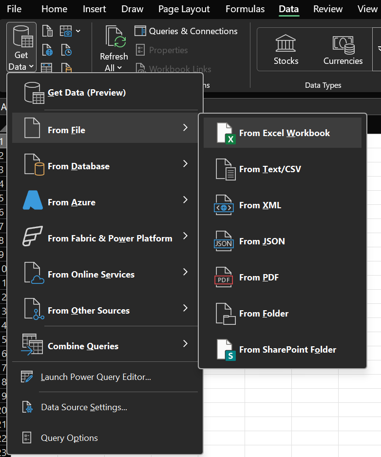 Figure 1a. Find the Excel Workbook connector to load data. |
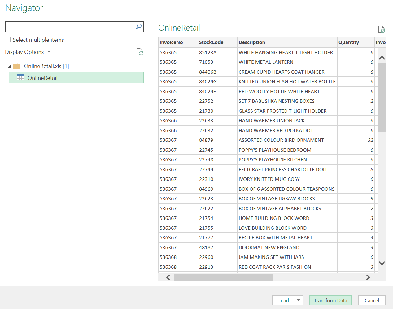 Figure 1b. Load the table into Power Query for processing. |
Right after loading, enable Column Quality and Column Distribution in the View tab.
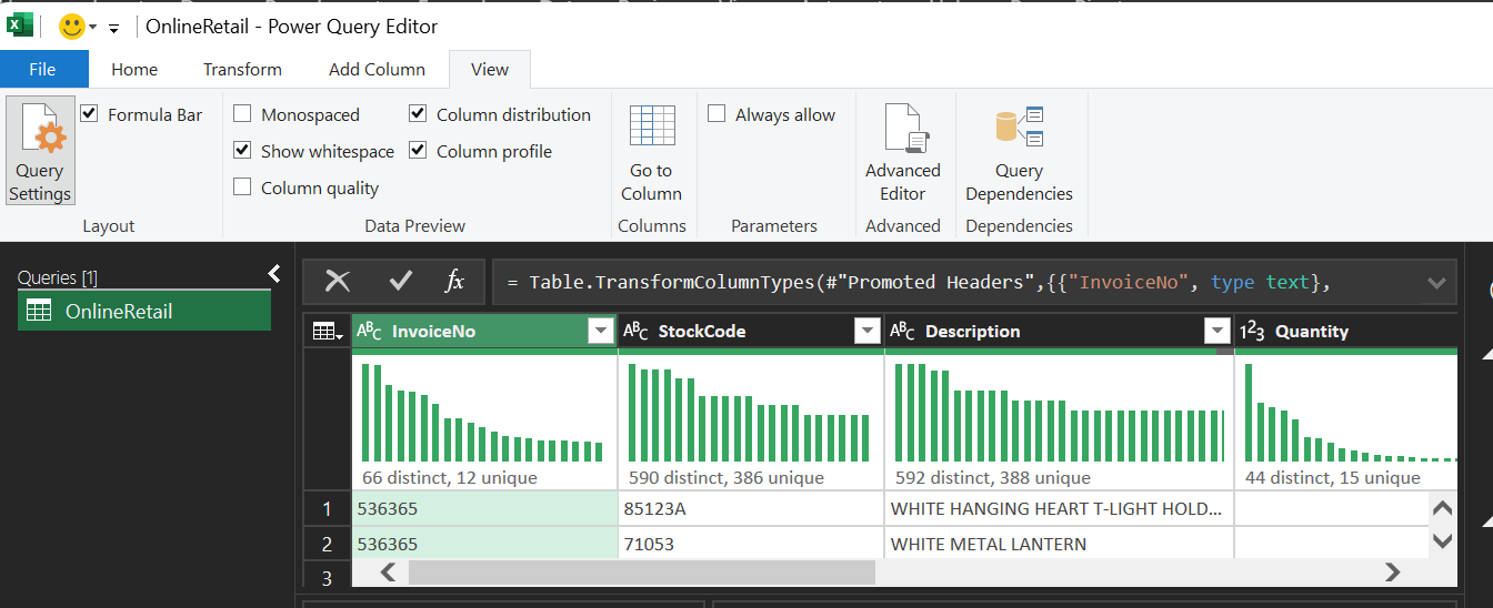
Figure 2. Open View and enable profiling tools (Column Quality/Distribution/Profile).
Enable quantitative checks at the source:
- Column Quality: check "Valid", "Error", and "Empty". The result shows CustomerID has only 75.1% valid values.
- Column Distribution: identify SKU distribution; notice non-product codes such as POST (postage), D (discount), M (manual).
- Column Profile: see min/max/mean; detect negative Quantity (returns) such as -80,995.
Column Profile view for min/max signals:
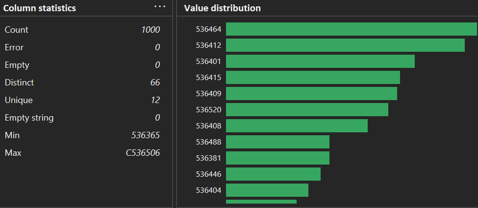
Figure 3. Check the bottom of Column statistics (Min/Max) to spot abnormal values early.
Step 2: Handle missing data
Analysis shows there are 135,080 rows missing customer identifiers.
- Action: right-click
CustomerID-> Remove Empty. - Why filtering out (instead of imputation)?
- Identity:
CustomerIDis the key to link transactions to customer behavior. Filling with a dummy value (e.g., 0) would incorrectly merge all those transactions into one customer, ruining retention/segmentation analysis. - RFM: Recency and Frequency computations require correct customer identity from CRM.
Result:
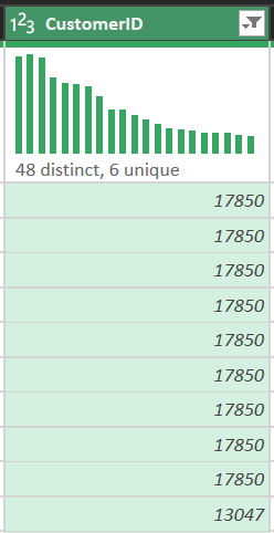
Figure 4. Removing empty CustomerID rows to preserve customer identity.
Step 3: Filter transaction noise
Raw data includes cancelled invoices (prefix C in InvoiceNo) and test rows.
- Action: set a combined filter so both
QuantityandUnitPriceare greater than 0. - Business meaning: remove cancelled orders, freebies (price 0), and invalid entries. This supports calculating Net Revenue rather than inflated numbers.
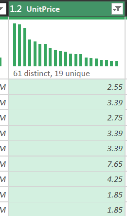
Figure 5. Use the filter icon to remove invalid transactions.
Step 4: Data typing (formatting)
Force types to optimize Excel Data Model performance:
- InvoiceDate: Date/Time (trend analysis by hour/month)
- UnitPrice: Decimal Number (preserve currency precision)
- Quantity: Whole Number
- CustomerID: Whole Number (as an identifier, not text)
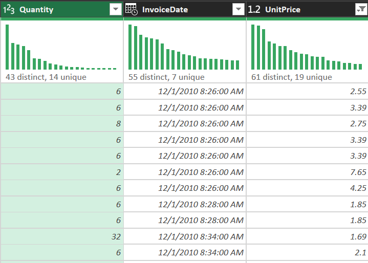
Figure 6. Set correct types for Quantity, InvoiceDate, and UnitPrice to avoid downstream issues.
Step 5: Text cleaning - normalize SKUs
The Description column often contains manual entry issues:
- Trim: remove leading/trailing spaces
- Clean: remove hidden characters
- Capitalize Each Word: consistent casing
Example: " red mug" -> "Red Mug"
Result: pivot tables won't split the same item into multiple variants due to spacing/casing.
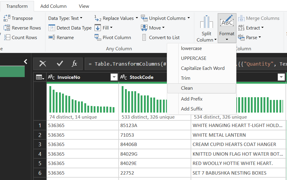
Figure 7. Use Format tools to normalize text (Trim/Clean/Capitalize Each Word).
Step 6: Add an order type column
Create a logic column to classify transaction scale:
- Action: Add Column -> Conditional Column
- Logic: if Quantity > 100 then "Wholesale" else "Retail"
- Purpose: support slicers and comparisons on the dashboard
Figure 8. Define a conditional rule to classify Wholesale vs Retail.
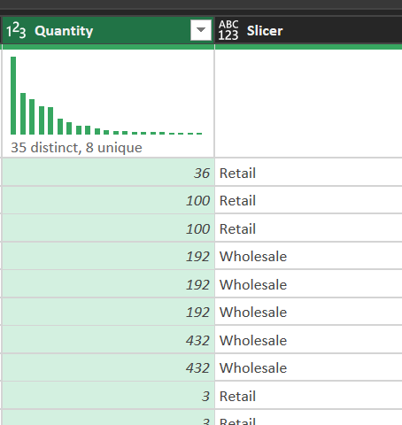
Figure 9. Verify the new order type column in the preview.
Step 7: Reuse the transformation history
All steps are recorded in the Applied Steps panel.
- Meaning: this becomes an automation "script". When next month's file arrives, simply click Refresh and Power Query replays the workflow consistently, eliminating manual errors and improving reproducibility.
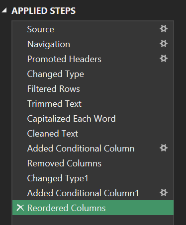
Figure 10. Applied Steps records the pipeline so it can be re-run with Refresh.
Step 8: Advanced Editor & M language
For the most complex work, use Advanced Editor to control the source code directly.
Full M-code example for the pipeline:
let
    Source = Excel.Workbook(File.Contents("C:\\Data\\OnlineRetail.xlsx"), null, true),
    Data = Source{[Item="Sheet1",Kind="Sheet"]}[Data],
    #"Promoted Headers" = Table.PromoteHeaders(Data, [PromoteAllScalars=true]),
    // Filter out noise and nulls in one step to optimize Query Folding
    #"CleanedData" = Table.SelectRows(#"Promoted Headers", each [CustomerID] <> null and [Quantity] > 0 and [UnitPrice] > 0),
    #"ChangedTypes" = Table.TransformColumnTypes(#"CleanedData",{
        {"Quantity", Int64.Type}, {"UnitPrice", type number}, {"CustomerID", Int64.Type}, {"InvoiceDate", type datetime}
    }),
    #"FormattedText" = Table.TransformColumns(#"ChangedTypes", {{"Description", each Text.Proper(Text.Trim(_)), type text}}),
    #"AddedStatus" = Table.AddColumn(#"FormattedText", "OrderType", each if [Quantity] > 100 then "Wholesale" else "Retail")
in
    #"AddedStatus"
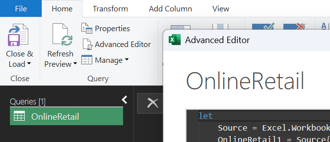
Figure 11. Open Advanced Editor to review and standardize the M-code pipeline.
3.2. Descriptive Statistics and the Analyst's Role
Use Excel's Descriptive Statistics to interpret the numbers behind the cleaned dataset.
Key metrics:
| Metric | Value | Interpretation |
|---|---:|---|
| MEAN | $22.39$ | Average revenue per line item |
| MEDIAN | $12.30$ | The typical "center" of the distribution |
| Std Dev $\sigma$ | $165.05$ | Dispersion driven by high-variance transactions |
| Skewness | $3.2$ | Right-skewed distribution; some very large orders exist |
Standard deviation formula:
$$ \sigma = \sqrt{\frac{1}{N} \sum_{i=1}^{N} (x_i - \mu)^2} $$
Why is the median a "lifesaver" here?
- In this dataset, wholesalers buying thousands of units create extreme outliers that inflate the mean. The median ($12.30$) is robust to outliers and better represents the "typical" behavior of the majority of retail customers.
3.3. Python (Pipeline Validation)
Python is used to validate the Power Query pipeline and ensure objective, reproducible results.
1. Setup
Libraries:
from pathlib import Path
import matplotlib.pyplot as plt
import pandas as pd
from google.colab import files
from IPython.display import display
Pandas display formatting:
pd.set_option("display.max_columns", None)
pd.set_option("display.float_format", lambda value: f"{value:,.2f}")
Upload the file to Colab and read it with pandas:
input_path = Path(next(iter(files.upload())))
raw_data = pd.read_excel(input_path, engine="xlrd")
Link csv: Download CSV data
2. Column naming
Use column names without spaces:
- NameName
- Name_Name
TEXT_COLUMNS = ["InvoiceNo", "StockCode", "Description", "Country"]

# Required columns for validity checks
REQUIRED_COLUMNS = [
    "InvoiceNo",
    "StockCode",
    "Description",
    "Quantity",
    "InvoiceDate",
    "UnitPrice",
    "Country",
]
3. Normalize text and empty values
def normalize_text(text_series: pd.Series) -> pd.Series:
    return (
        # Convert to string
        text_series.astype("string")
        # Remove extra whitespace
        .str.replace(r"\\s+", " ", regex=True)
        .str.strip()
        # Treat empty strings as missing values
        .replace({"": pd.NA, "<NA>": pd.NA})
    )
4. Build a before/after report
Create a summary table to compare metrics before and after cleaning:
def build_report(data_frame: pd.DataFrame) -> pd.DataFrame:
    summary_values = {
        "total_rows": len(data_frame),
        "missing_customer_id": data_frame["CustomerID"].isna().sum(),
        "cancelled_invoices": data_frame["InvoiceNo"].str.startswith("C", na=False).sum(),
        "non_positive_quantity": data_frame["Quantity"].le(0).sum(),
        "non_positive_unit_price": data_frame["UnitPrice"].le(0).sum(),
        "duplicate_rows": data_frame.duplicated().sum(),
        "gross_sales": round(data_frame["SaleAmount"].fillna(0).sum(), 2),
        "mean_quantity": round(data_frame["Quantity"].dropna().mean(), 2),
        "median_quantity": round(data_frame["Quantity"].dropna().median(), 2),
        "mean_unit_price": round(data_frame["UnitPrice"].dropna().mean(), 2),
        "median_unit_price": round(data_frame["UnitPrice"].dropna().median(), 2),
        "mean_sale_amount": round(data_frame["SaleAmount"].dropna().mean(), 2),
        "median_sale_amount": round(data_frame["SaleAmount"].dropna().median(), 2),
    }

    return pd.DataFrame(summary_values.items(), columns=["metric", "value"])
Result (before vs. after):
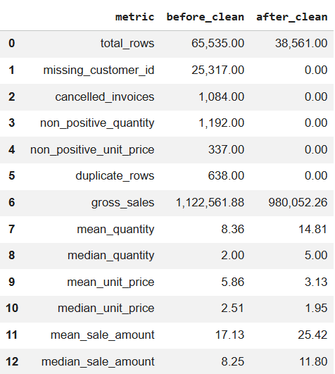 Figure 12a. Metrics before cleaning. |
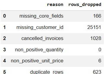 Figure 12b. Metrics after cleaning. |
5. Clean the data
def clean_online_retail(raw_data: pd.DataFrame):
    # Copy raw data to avoid in-place edits
    cleaned_data = raw_data.copy()

    # Normalize text columns (dedupe whitespace, standardize)
    for column_name in TEXT_COLUMNS:
        cleaned_data[column_name] = normalize_text(cleaned_data[column_name])

    # Normalize CustomerID: e.g., 123.0 -> 123
    cleaned_data["CustomerID"] = normalize_text(cleaned_data["CustomerID"]).str.replace(
        r"\\.0$", "", regex=True
    )

    # Coerce types
    cleaned_data["Quantity"] = pd.to_numeric(
        cleaned_data["Quantity"], errors="coerce"
    ).astype("Int64")
    cleaned_data["UnitPrice"] = pd.to_numeric(cleaned_data["UnitPrice"], errors="coerce")
    cleaned_data["InvoiceDate"] = pd.to_datetime(
        cleaned_data["InvoiceDate"], errors="coerce"
    )

    # Row-level sales amount
    cleaned_data["SaleAmount"] = (
        cleaned_data["Quantity"].astype("float") * cleaned_data["UnitPrice"]
    ).round(2)

    # Before-cleaning report
    before_table = build_report(cleaned_data).rename(columns={"value": "before_clean"})

    # Rules for invalid rows
    invalid_rules = [
        ("missing_core_fields", cleaned_data[REQUIRED_COLUMNS].isna().any(axis=1)),
        ("missing_customer_id", cleaned_data["CustomerID"].isna()),
        ("cancelled_invoices", cleaned_data["InvoiceNo"].str.startswith("C", na=False)),
        ("non_positive_quantity", cleaned_data["Quantity"].le(0)),
        ("non_positive_unit_price", cleaned_data["UnitPrice"].le(0)),
    ]

    keep_row = pd.Series(True, index=cleaned_data.index)
    removed_rows = []

    for rule_name, invalid_row in invalid_rules:
        current_removed_row = keep_row & invalid_row
        removed_rows.append((rule_name, int(current_removed_row.sum())))
        keep_row &= ~invalid_row

    # Drop duplicates after filtering
    final_data = cleaned_data.loc[keep_row].drop_duplicates().copy()
    duplicate_rows = int(cleaned_data.loc[keep_row].duplicated().sum())

    # Sort
    final_data = final_data.sort_values(
        ["InvoiceDate", "InvoiceNo", "StockCode"]
    ).reset_index(drop=True)

    # After-cleaning report
    after_table = build_report(final_data).rename(columns={"value": "after_clean"})
    comparison_table = before_table.merge(after_table, on="metric")

    removed_table = pd.DataFrame(
        removed_rows + [("duplicate_rows", duplicate_rows)],
        columns=["reason", "rows_dropped"],
    )

    return final_data, comparison_table, removed_table
6. Visualize mean vs. median
# Count metrics (row counts and error counts)
count_metrics = [
    "total_rows",
    "missing_customer_id",
    "cancelled_invoices",
    "duplicate_rows",
]

# Value metrics (mean/median trends)
value_metrics = [
    "mean_quantity",
    "median_quantity",
    "mean_unit_price",
    "median_unit_price",
    "mean_sale_amount",
    "median_sale_amount",
]

figure, axes = plt.subplots(1, 2, figsize=(14, 5))

# Chart 1: count metrics before vs after
comparison_table[comparison_table["metric"].isin(count_metrics)].set_index("metric")[
    ["before_clean", "after_clean"]
].plot(kind="bar", ax=axes[0], color=["#d97706", "#15803d"])
axes[0].set_title("Count Metrics")
axes[0].set_xlabel("")
axes[0].set_ylabel("Count")
axes[0].tick_params(axis="x", rotation=0)

# Chart 2: mean vs median before vs after
comparison_table[comparison_table["metric"].isin(value_metrics)].set_index("metric")[
    ["before_clean", "after_clean"]
].plot(kind="bar", ax=axes[1], color=["#2563eb", "#16a34a"])
axes[1].set_title("Mean and Median")
axes[1].set_xlabel("")
axes[1].set_ylabel("Value")
axes[1].tick_params(axis="x", rotation=45)

plt.tight_layout()
plt.show()
Result:
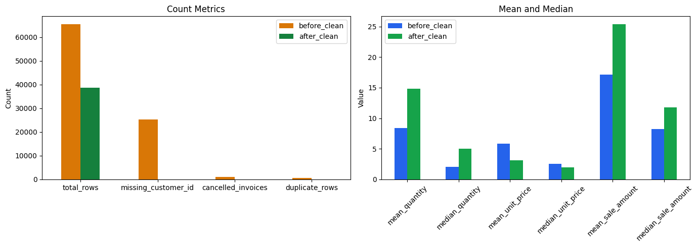
Figure 13. Before/after comparison for key metrics and mean/median values.
7. Export files
output_folder = Path("/content/output")
output_folder.mkdir(parents=True, exist_ok=True)

# Export datetime in a consistent format
export_data = clean_data.copy()
export_data["InvoiceDate"] = export_data["InvoiceDate"].dt.strftime("%Y-%m-%d %H:%M:%S")

# Export CSVs
export_data.to_csv(
    output_folder / "online_retail_clean.csv",
    index=False,
    encoding="utf-8-sig",
)
comparison_table.to_csv(
    output_folder / "before_after_summary.csv",
    index=False,
    encoding="utf-8-sig",
)
removed_table.to_csv(
    output_folder / "dropped_reason_summary.csv",
    index=False,
    encoding="utf-8-sig",
)

list(output_folder.iterdir())
4. Conclusion
Data quality directly determines the reliability of analytics (GIGO). In omnichannel retail, a clear, repeatable cleaning pipeline is essential so that metrics such as revenue, customer behavior, and segmentation reflect reality.
In this post, Power Query serves as a practical visual ETL tool to standardize data through an 8-step workflow. Python acts as an independent validation layer to reproduce the logic, generate before/after comparisons, and improve objectivity. Once the input data is clean and consistent, descriptive statistics and dashboarding become more stable and decision risk decreases.
5. References
[1] Kaggle, Online Retail Dataset. https://www.kaggle.com/datasets/lakshmi25npathi/online-retail-dataset
[2] OnlineRetail.csv, practice data file used in this project (downloaded from Kaggle and converted to CSV).
[3] Microsoft Learn, Power Query. https://learn.microsoft.com/power-query/
[4] Microsoft Learn, Power Query M formula language. https://learn.microsoft.com/powerquery-m/
[5] pandas Documentation. https://pandas.pydata.org/docs/
[6] Matplotlib Documentation. https://matplotlib.org/stable/
[7] Wikipedia, Garbage in, garbage out. https://en.wikipedia.org/wiki/Garbage_in,_garbage_out
Chưa có bình luận nào. Hãy là người đầu tiên!