
I. INTRODUCTION
In countries with a large number of motorcycles such as Vietnam, mandatory helmet use is one of the key measures to reduce traumatic brain injuries and fatalities caused by traffic accidents. However, manual inspection by traffic enforcement officers is limited in terms of manpower, cost, and spatiotemporal coverage. The development of Deep Learning and YOLO models enables the construction of automatic surveillance systems capable of detecting motorcyclists and assessing their helmet-wearing status in real time from traffic camera video streams.
In this project, we build upon prior works on helmet violation detection using YOLOv5/YOLOv8 and deploy the approach on YOLOv11, a new generation with an architecture optimized for accuracy and efficiency. The objective is to construct a complete pipeline from data preparation, model training and evaluation to demonstrating its applicability in real-world scenarios (e.g., monitoring a motorcycle lane with a fixed camera).
II. LITERATURE REVIEW
Recently, many studies have applied computer vision and deep learning to automatically detect traffic law violations from surveillance camera data. Systems based on convolutional neural networks (CNN) can accurately recognize violations such as riding a motorcycle without a helmet, running red lights, driving in the wrong lane (lane encroachment or wrong-way driving), and various other dangerous behaviors. Compared with traditional manual methods, these artificial intelligence (AI) models provide higher accuracy and can operate continuously 24/7, thereby improving traffic monitoring effectiveness. For example, Deshpande et al [1] proposed a two-stage deep learning system to detect motorcycle riders without helmets: first detecting two‑wheelers using DetectNet (ResNet18), then using YOLOv8 to check whether the rider is wearing a helmet. This system achieves helmet detection accuracy of up to ~98.5% and is designed for real-time operation, helping to reduce the workload of traffic police in monitoring violations. Similarly, Adi et al [2] developed a violation detection system for two‑wheel vehicles using Faster R‑CNN, which can simultaneously detect no‑helmet violations and lane-mark violations (lane encroachment or line crossing) with an accuracy of about 85%. These results demonstrate that CNN-based object recognition is highly effective in complex traffic environments. For red-light running behavior, a common approach is to combine traffic light recognition with vehicle tracking. Specifically, Thao et al [3] used the YOLOv5s model (a small variant of YOLOv5) fine-tuned on the COCO dataset to detect signal light states and vehicle positions, thereby automatically determining red‑light violations. Their system achieves ~90% accuracy in recognizing light states and ~86% in detecting red‑light violations. In addition, several studies integrate object tracking algorithms to analyze vehicle motion behavior. Dede et al [4] introduced an intelligent surveillance system that integrates YOLOv5 to detect entities (cars, pedestrians, traffic lights, signs, etc.) and the StrongSORT tracking algorithm to track their trajectories. After detection and tracking, the system applies specific analysis algorithms for each violation type—for example, determining whether a vehicle runs a red light based on its position relative to the stop line when the light is red, detecting vehicles entering the emergency lane or driving in the wrong lane based on comparing trajectories with lane markings, and so on. Using this approach, the system of Dede et al. automatically detects six common violations (including red‑light running, entering the emergency lane, not keeping safe distance, crosswalk violations, and illegal parking) and extracts license plates with OCR to support enforcement. These advances confirm that applying deep learning and image processing techniques in traffic surveillance is not only feasible but also achieves high accuracy, enabling timely detection of dangerous violations to enhance road safety.
III. RESOURCES AND METHODS
3.1. Data collection and preprocessing
The dataset used in this study is constructed from frames extracted from traffic videos, where each image contains one or more motorcycles moving on the road. Objects are annotated with three categories: license plate, rider with helmet, and rider without helmet, forming a total of 1,340 bounding boxes. The data is split into training and validation sets (e.g., 80/20), ensuring that class distribution across subsets is relatively balanced to reduce bias during training.
3.2. Hyperparameter setup for the YOLOv11 model
The model is built on the YOLOv11 architecture developed by Ultralytics, initialized from pretrained weights on the COCO dataset to leverage general feature extraction capabilities. The hyperparameters are selected to ensure stable convergence under limited hardware conditions while maintaining acceptable object detection quality for real-world applications.
In addition, we apply early stopping and save the best checkpoint according to mAP on the validation set to avoid overfitting. Training is conducted in Python using the integrated Ultralytics training pipeline, which automatically logs loss, mAP, precision, and recall metrics and plots learning curves for post‑training analysis.
3.3. Experimental environment
Model training is performed on a workstation running Microsoft Windows 10 Pro 64‑bit (version 19045), built on a Colorful BATTLE‑AX B760M‑K D5 system (BIOS version 1009) and equipped with an Intel Core i5‑14600KF processor (20 logical CPUs) and 32 GB of RAM. To accelerate computation, the system uses an NVIDIA GeForce RTX 5070 GPU with 11,854 MB of VRAM (approximately 28,151 MB total graphics memory including shared memory) and supports DirectX 12. The training pipeline is implemented in Python using the Ultralytics YOLO (YOLOv11) framework, along with PyTorch‑based components (e.g., Swin Transformer via timm) and image processing/augmentation libraries such as OpenCV and Albumentations, providing a powerful foundation for handling the computational demands of deep learning training and inference.
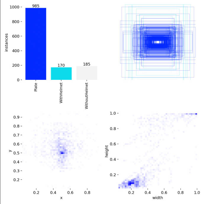
Figure 1. Statistics and label distribution in the dataset
| No. | Label type | Quantity |
|---|---|---|
| 1 | License plate | 985 |
| 2 | With helmet | 170 |
| 3 | Without helmet | 185 |
| Total | 1340 | |
Table 1. Number of labels and distribution
3.4. Proposed method
The proposed method builds a real-time helmet‑violation detection system based on YOLOv11, optimized for realistic traffic conditions (day/night, rain/sun, motion blur, speed‑induced blur). The system consists of three main modules:
- Context recognition of weather/illumination from video frames to drive data augmentation strategies and improve robustness.
- Multi‑stage fine‑tuning of YOLOv11 to ensure stable convergence and reduce dependence on mosaic augmentation in the final training phase.
- Enhanced inference using Test‑Time Augmentation (TTA) and prediction fusion via NMS to reduce missed detections in difficult cases.
In this task, the model simultaneously detects three target classes:
- Plate: license plate,
- WithHelmet: rider with helmet,
- WithoutHelmet: rider without helmet.
The classes are annotated with bounding boxes and used directly for violation detection.
To better adapt to diverse environmental conditions, we add a weather/illumination classification module based on the Swin Transformer (Swin‑Tiny) backbone. This module predicts four context states: day_clear, day_rainy, night_clear, and night_rainy.
For frames classified as *_rainy, the system activates “synthetic rain” augmentation using Albumentations RandomRain to simulate rain streaks and degraded visibility.
For all states, standard augmentations are applied: horizontal flipping, brightness/contrast adjustment, Gaussian blur, and region‑wise dropout (coarse dropout) to simulate partial occlusion and camera noise.
This mechanism helps the training data distribution better reflect real‑world conditions, especially in rainy/night scenarios that often degrade detection quality.
In traffic surveillance, videos are typically very long and contain many redundant frames. To optimize data costs, the proposed method adopts few‑shot sampling to select a representative subset of frames before annotation/training:
- From each video, select at most N frames (e.g., N = 1000) using uniform temporal sampling or a combination with change‑based criteria (difference between consecutive frames).
- The objective is to ensure diversity in camera angle, distance, lighting conditions, traffic density, and helmet/no‑helmet situations.
This sampling strategy significantly reduces the number of images requiring manual processing while preserving sufficient scenario coverage for training.
3.5. Model training
The object detection model is built using Ultralytics YOLOv11.
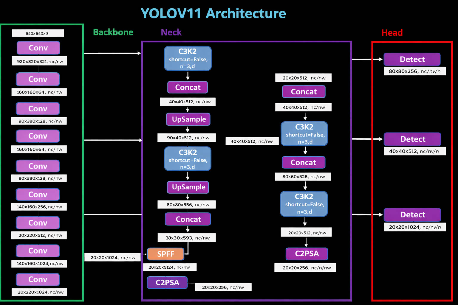
Figure 2. YOLOv11 model architecture
| Hyperparameter | Value |
|---|---|
| Batch size | batch = 16 |
| Image size | 640 × 640 pixels |
| Number of epochs | 100 |
| Optimizer | AdamW |
| Learning rate | 0.01 |
Table 2. Hyperparameters used for model training
In this study, we train YOLOv11 following the backbone–neck–head architecture (see the YOLOv11 architecture figure) to simultaneously detect license plates, helmeted riders, and non‑helmeted riders from traffic video frames. Before training, the data is cleaned, resized, and split into train/validation/test subsets with appropriate ratios to ensure objective evaluation. We also apply data augmentation techniques (horizontal flipping, brightness–contrast adjustment, slight blur, noise, and local occlusion; for rainy frames, additional rain simulation) to improve generalization in real‑world conditions such as rain/night and motion blur. The model is initialized from pretrained weights to shorten convergence time and enhance performance on the limited dataset. Training is conducted with an experimental configuration of image size = 640, batch size = 16, AdamW optimizer with initial learning rate lr0 = 0.01, mixed‑precision enabled to optimize speed and memory, and approximately 100 epochs following a multi‑stage strategy. In the fine‑tuning phase, mosaic augmentation is disabled in the last epochs (e.g., close_mosaic = 10) to help the model learn boundary details and small objects more stably under complex conditions. During training, the system continuously monitors loss and validation metrics, automatically saving the best weights (best.pt) based on overall detection quality, and finally evaluates the model using standard object detection metrics such as Precision, Recall, F1‑score, mAP50, and mAP50‑95, along with visual checks using the confusion matrix and PR curves to validate model reliability before real‑time deployment with the Ultralytics framework.
3.6. Model evaluation
To evaluate the detection quality, we compare predicted bounding boxes with ground truth using Intersection over Union (IoU) (1). A prediction is considered correct (True Positive – TP) when IoU exceeds a threshold τ (e.g., τ = 0.5); otherwise, unmatched predictions are treated as False Positives (FP), and ground‑truth objects not detected are False Negatives (FN). Based on this, the model is evaluated using Precision (2), Recall (3), F1‑score (4), and mAP‑based metrics (AP and mAP). Here, mAP50 reflects detection performance at IoU = 0.5, while mAP50‑95 provides a more comprehensive measure by averaging over multiple IoU thresholds.
$$IoU = \frac{\mid B_{pred} \cup B_{gt} \mid}{\mid B_{pred} \cap B_{gt} \mid}\ (1)$$
$$P = \frac{TP}{TP + FP} (2)$$
$$R = \frac{TP}{TP + FN} (3)$$
$$F1 = \frac{2PR}{P + R} = \frac{2TP}{2TP + FP + FP}(4)$$
Next, to assess model quality across all confidence thresholds, we construct the Precision–Recall curve (5) and compute the Average Precision (AP) (6) for each class. In many studies, AP is estimated using 11‑point interpolation, where precision at each normalized recall level $r \in \{ 0,0.1,\ldots,1.0\}$) is interpolated by the maximum precision achieved at any recall $\widetilde{r}\geq r$.
$$P_{interp}(r) = \max_{\widetilde{r} \geq r}{ P\left( \widetilde{r} \right)} (5)$$
$$AP = \frac{1}{11}\sum_{ r \in \{ 0,0.1,\ldots,1.0\}}^{} P_{interp}(r) (6)$$
Then, the mean Average Precision (mAP) is computed as the average of AP over all classes, reflecting the overall performance of the model on the full set of target objects. Specifically, for each class $i$), AP is estimated via 11‑point interpolation on the Precision–Recall curve by averaging precision values at normalized recall levels $R_{i}$) as shown in (6). Using 11‑point averaging stabilizes the metric and reduces the effect of local fluctuations on the PR curve when changing the confidence threshold. After obtaining $AP_{i}$) for each class, mAP is defined as the arithmetic mean of all $AP_{i}$) across the number of classes, as in (7). Thus, mAP not only captures single‑class performance but also provides a global metric that enables fair comparison between models under the same data and evaluation settings.
$$mAP = \frac{1}{classes}\sum_{i = 1}^{classes}{AP_{i}} (7)$$
IV. RESULTS
4.1. Experimental results
The convergence behavior of the model is illustrated by the training and validation curves (Figure 3). The results show that train/box_loss, train/cls_loss, and train/dfl_loss decrease steadily over epochs; similarly, val/box_loss, val/cls_loss, and val/dfl_loss also decrease and stabilize after initial fluctuations, indicating that the model learns meaningful features without severe train–validation divergence. Regarding performance metrics, Precision and Recall increase rapidly in the early epochs and then stabilize, while mAP50 and mAP50‑95 gradually increase and saturate in the final stage, suggesting that the model reaches a suitable convergence state for selecting the best checkpoint for inference.
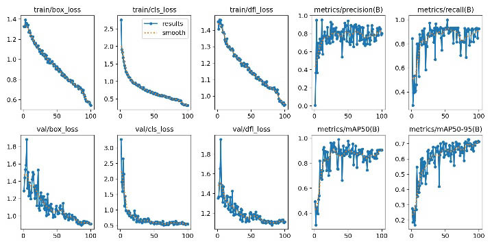
Figure 3. Training and evaluation results of the YOLOv11 model
Additionally, confidence‑based plots (Figure 4) provide a basis for choosing operating thresholds: the F1–Confidence curve peaks at approximately 0.85 at a confidence threshold of about 0.279, corresponding to a good balance between Precision and Recall. Meanwhile, the Recall–Confidence curve (Figure 5) drops sharply as confidence increases (especially beyond ~0.8), reflecting the typical trade‑off between reducing false positives and increasing missed detections.
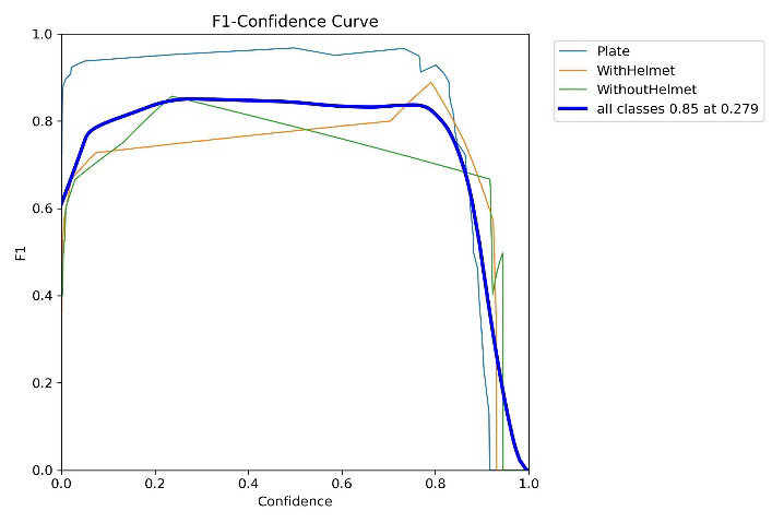
Figure 4. F1–Confidence evaluation
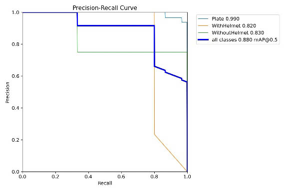
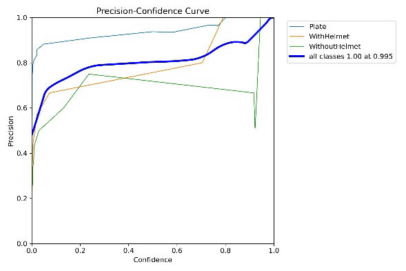
Figure 5. Precision–Confidence and Recall–Confidence
The confusion matrix (Figure 6) shows that the Plate class is detected very reliably (30 correct predictions), but there are still some misclassifications as background and mutual confusion between WithHelmet and WithoutHelmet. This is the main factor reducing the precision of the two helmet‑related classes in challenging situations (oblique viewpoints, occlusions, low image quality).
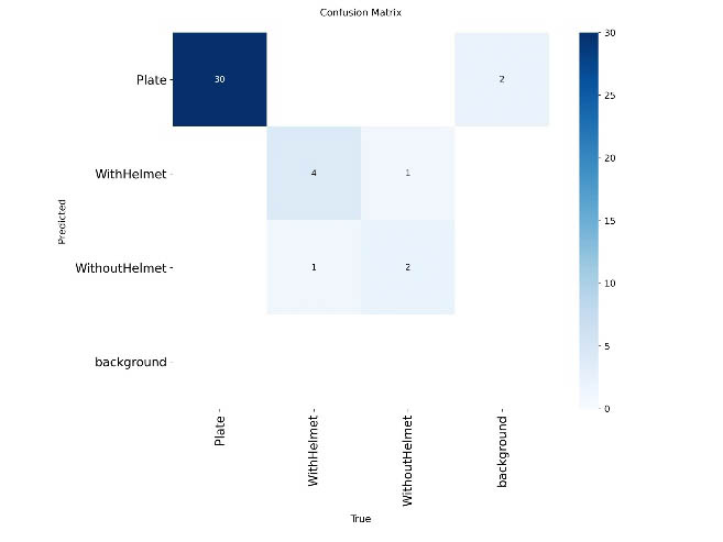
Figure 6. Confusion matrix
4.2. Test results
On the test set, the model achieves overall performance of Precision = 0.798, Recall = 0.913, mAP50 = 0.9109, mAP50‑95 = 0.6610, and mAP75 = 0.7656, indicating strong detection capability at the standard IoU threshold and reasonably good localization when stricter criteria are applied. The F1 score aggregated from Precision–Recall is approximately 0.852, consistent with the observed peak on the F1–Confidence curve. By class, Plate achieves P = 0.925, R = 0.967, mAP50 = 0.983, mAP50‑95 = 0.651 (F1 ≈ 0.946), showing high reliability for evidence extraction. WithHelmet achieves P = 0.726, R = 0.800, mAP50 = 0.920, mAP50‑95 = 0.679 (F1 ≈ 0.761), and WithoutHelmet achieves P = 0.743, R = 0.973, mAP50 = 0.830, mAP50‑95 = 0.654 (F1 ≈ 0.843). The very high recall of WithoutHelmet aligns with the goal of minimizing missed violations, though precision still needs improvement to reduce false alarms.
Regarding real-time deployment capability, the average processing time is ~1.2 ms for preprocessing, ~26.5 ms for inference, and ~0.5 ms for post‑processing per image (total ~28.2 ms/frame, equivalent to about 35 FPS), satisfying continuous video surveillance requirements. The system output includes annotated frames (bounding boxes, classes, and confidence scores) and can store evidence when WithoutHelmet is detected, with priority extraction of the corresponding Plate region to support subsequent steps (storage, cross‑checking, OCR), thereby completing the helmet‑violation detection workflow in real traffic settings.
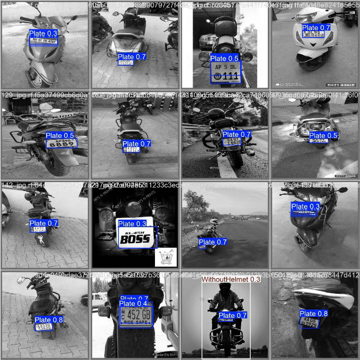
Figure 7. Sample training images
V. CONCLUSION
This study proposes and successfully implements a helmet‑violation detection system for traffic environments based on the YOLOv11 model, integrated with an evaluation pipeline using standard object‑detection metrics. Experimental results show promising overall performance with Precision = 0.798, Recall = 0.913, mAP50 = 0.9109, mAP50‑95 = 0.6610, and mAP75 = 0.7656, reflecting strong detection at the standard IoU threshold and reasonably good localization when stricter evaluation levels are applied. In particular, the Plate class attains high reliability (mAP50 = 0.983), effectively supporting evidence extraction, while the WithoutHelmet class achieves very high Recall (0.973), reducing the risk of missed violations - an important requirement for surveillance and enforcement systems.
Moreover, confidence‑based analysis shows that the F1‑score peaks at ~0.85 at a confidence of approximately 0.279, providing a basis for selecting an operating threshold that balances false positives and missed detections. The processing speed of ~28.2 ms/frame (~35 FPS) demonstrates that the system can meet real‑time requirements. However, due to the limited number of test samples for helmet‑related classes, class‑wise metrics may fluctuate and should be reinforced with larger and more diverse datasets (nighttime, rain, oblique angles, occlusions, high traffic density) to increase statistical reliability.
VI. FUTURE WORK
In the future, a natural development direction is to expand the dataset with more diverse scenarios (nighttime, rain, fog, high traffic density) to improve model generalization. Additionally, integrating an automatic number plate recognition (ANPR) module and linking it with enforcement databases will turn the violation detection model into a complete system supporting law enforcement. Finally, model optimization and compression techniques (quantization, pruning) can be investigated to enable deployment on resource‑constrained edge devices such as smart cameras or on‑site processing units.
VII. REFERENCES
- Deshpande, U. U., Michael, G. K. O., Araujo, S. D. C. S., Deshpande, V., Patil, R., Chate, R. A. A., Tandur, V. R., Goudar, S. S., Ingale, S., & Charantimath, V. (2025). Computer-vision based automatic rider helmet violation detection and vehicle identification in Indian smart city scenarios using NVIDIA TAO toolkit and YOLOv8. Frontiers in Artificial Intelligence, 8, Article 1582257. https://doi.org/10.3389/frai.2025.1582257
- Adi, K., Widodo, C. E., Widodo, A. P., & Masykur, F. (2024). Traffic violation detection system on two-wheel vehicles using convolutional neural network method. TEM Journal, 13(1), 531–536. https://doi.org/10.18421/TEM131-55
- Le, Q. T., Duong, D. C., Nguyen, T. A., Pham, M. A., Ha, M. D., & Nguyen, M. (2022). Automatic traffic red-light violation detection using AI. Ingénierie des Systèmes d’Information, 27(1), 75–80. https://doi.org/10.18280/isi.270109
- Dede, D., Sarsıl, M. A., Shaker, A., Altıntaş, O., & Ergen, O. (2023). Next-gen traffic surveillance: AI-assisted mobile traffic violation detection system. arXiv preprint, arXiv:2311.16179. https://doi.org/10.48550/arXiv.2311.16179
Chưa có bình luận nào. Hãy là người đầu tiên!